Bayesian Decision Making for Continuous Endpoints

library(BayesianQDM)
library(dplyr)
#> 
#> Attaching package: 'dplyr'
#> The following objects are masked from 'package:stats':
#> 
#>     filter, lag
#> The following objects are masked from 'package:base':
#> 
#>     intersect, setdiff, setequal, union
library(tidyr)
library(ggplot2)
library(purrr)

Introduction

This vignette demonstrates Bayesian decision-making for continuous endpoints using the BayesianQDM package. Continuous endpoints (e.g., change in biomarker levels, symptom scores, or quality of life measures) are common in clinical trials and require different statistical approaches than binary endpoints.

Theoretical Background

Statistical Framework

For continuous endpoints, we assume: - Outcomes follow normal distributions with unknown means and variances - Prior distributions on parameters (Normal-Inverse-Chi-squared or vague priors) - Posterior distributions follow t-distributions

Calculation Methods

The package provides three computational approaches:

1. NI (Numerical Integration): Exact calculation using convolution
2. WS (Welch-Satterthwaite): Fast approximation for unequal variances
   
3. MC (Monte Carlo): Simulation-based approach

For this vignette, we focus on the fastest methods (NI and WS) to ensure reasonable build times.

Basic Examples

Posterior Probability

# Calculate posterior probability using NI method
posterior_prob <- pPPsinglecontinuous(
  prob = 'posterior', 
  design = 'controlled', 
  prior = 'vague', 
  CalcMethod = 'NI',
  theta0 = 1.5,
  n1 = 20, n2 = 20, 
  bar.y1 = 5.2, bar.y2 = 3.0, 
  s1 = 2.0, s2 = 1.8
)

cat("Posterior probability that treatment effect > 1.5:", round(posterior_prob, 4))
#> Posterior probability that treatment effect > 1.5: 0.1323

Comparing Calculation Methods

# Compare NI and WS methods
prob_ni <- pPPsinglecontinuous(
  prob = 'posterior', design = 'controlled', prior = 'vague', CalcMethod = 'NI',
  theta0 = 1.5, n1 = 15, n2 = 15, bar.y1 = 5, bar.y2 = 3, s1 = 2, s2 = 2
)

prob_ws <- pPPsinglecontinuous(
  prob = 'posterior', design = 'controlled', prior = 'vague', CalcMethod = 'WS',
  theta0 = 1.5, n1 = 15, n2 = 15, bar.y1 = 5, bar.y2 = 3, s1 = 2, s2 = 2
)

cat("NI method:", round(prob_ni, 4), "\n")
#> NI method: 0.2572
cat("WS method:", round(prob_ws, 4), "\n")
#> WS method: 0.2496
cat("Difference:", round(abs(prob_ni - prob_ws), 6), "\n")
#> Difference: 0.00763

Go/NoGo/Gray Decision Probabilities

Basic Usage

# Calculate Go/NoGo/Gray probabilities
result <- pGNGsinglecontinuous(
  nsim = 50,  # Small nsim for vignette speed
  prob = 'posterior', 
  design = 'controlled', 
  prior = 'vague', 
  CalcMethod = 'WS',
  theta.TV = 1.5, theta.MAV = 0.5, theta.NULL = NULL,
  nMC = NULL, gamma1 = 0.8, gamma2 = 0.3,
  n1 = 20, n2 = 20, m1 = NULL, m2 = NULL,
  kappa01 = NULL, kappa02 = NULL, nu01 = NULL, nu02 = NULL,
  mu01 = NULL, mu02 = NULL, sigma01 = NULL, sigma02 = NULL,
  mu1 = 5.0, mu2 = 3.0, sigma1 = 2.0, sigma2 = 1.8,
  r = NULL, ne1 = NULL, ne2 = NULL, alpha01 = NULL, alpha02 = NULL,
  bar.ye1 = NULL, bar.ye2 = NULL, se1 = NULL, se2 = NULL,
  seed = 123
)

print(result)
#>   mu1 mu2   Go Gray NoGo
#> 1   5   3 0.46 0.52 0.02

Operating Characteristics

Evaluating Across Treatment Effects

# Evaluate OC across different treatment effects
mu1_values <- seq(3, 7, by = 1)

oc_results <- do.call(rbind, lapply(mu1_values, function(m1) {
  result <- pGNGsinglecontinuous(
    nsim = 30,  # Reduced for vignette speed
    prob = 'posterior', design = 'controlled', prior = 'vague', CalcMethod = 'WS',
    theta.TV = 1.5, theta.MAV = 0.5, theta.NULL = NULL,
    nMC = NULL, gamma1 = 0.8, gamma2 = 0.3,
    n1 = 30, n2 = 30, m1 = NULL, m2 = NULL,
    kappa01 = NULL, kappa02 = NULL, nu01 = NULL, nu02 = NULL,
    mu01 = NULL, mu02 = NULL, sigma01 = NULL, sigma02 = NULL,
    mu1 = m1, mu2 = 3, sigma1 = 2, sigma2 = 2,
    r = NULL, ne1 = NULL, ne2 = NULL, alpha01 = NULL, alpha02 = NULL,
    bar.ye1 = NULL, bar.ye2 = NULL, se1 = NULL, se2 = NULL,
    seed = 123
  )
  
  data.frame(
    mu1 = m1,
    treatment_effect = m1 - 3,
    go_prob = result$Go,
    nogo_prob = result$NoGo,
    gray_prob = result$Gray
  )
}))

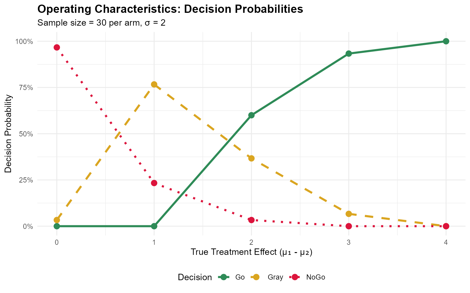
print(oc_results)
#>   mu1 treatment_effect   go_prob  nogo_prob  gray_prob
#> 1   3                0 0.0000000 0.96666667 0.03333333
#> 2   4                1 0.0000000 0.23333333 0.76666667
#> 3   5                2 0.6000000 0.03333333 0.36666667
#> 4   6                3 0.9333333 0.00000000 0.06666667
#> 5   7                4 1.0000000 0.00000000 0.00000000

Visualizing Operating Characteristics

# Reshape for plotting
plot_data <- oc_results %>%
  pivot_longer(cols = c(go_prob, gray_prob, nogo_prob), 
               names_to = "decision", 
               values_to = "probability") %>%
  mutate(Decision = case_when(
    decision == "go_prob" ~ "Go",
    decision == "gray_prob" ~ "Gray",
    decision == "nogo_prob" ~ "NoGo"
  ))

ggplot(plot_data, aes(x = treatment_effect, y = probability, color = Decision, linetype = Decision)) +
  geom_line(linewidth = 1.2) +
  geom_point(size = 3) +
  scale_color_manual(values = c("Go" = "#2E8B57", "Gray" = "#DAA520", "NoGo" = "#DC143C")) +
  scale_linetype_manual(values = c("Go" = "solid", "Gray" = "dashed", "NoGo" = "dotted")) +
  labs(
    title = "Operating Characteristics: Decision Probabilities",
    subtitle = "Sample size = 30 per arm, σ = 2",
    x = "True Treatment Effect (μ₁ - μ₂)",
    y = "Decision Probability",
    color = "Decision"
  ) +
  scale_y_continuous(limits = c(0, 1), labels = scales::percent) +
  theme_minimal() +
  theme(
    plot.title = element_text(face = "bold", size = 14),
    legend.position = "bottom"
  )

Prior Specification

Informative vs Vague Priors

# Vague prior
prob_vague <- pPPsinglecontinuous(
  prob = 'posterior', design = 'controlled', prior = 'vague', CalcMethod = 'NI',
  theta0 = 1.5, n1 = 15, n2 = 15, bar.y1 = 5, bar.y2 = 3, s1 = 2, s2 = 2
)

# Informative prior (Normal-Inverse-Chi-squared)
prob_informative <- pPPsinglecontinuous(
  prob = 'posterior', design = 'controlled', prior = 'N-Inv-Chisq', CalcMethod = 'NI',
  theta0 = 1.5, n1 = 15, n2 = 15,
  kappa01 = 5, kappa02 = 5, nu01 = 10, nu02 = 10,
  mu01 = 5, mu02 = 3, sigma01 = 2, sigma02 = 2,
  bar.y1 = 5, bar.y2 = 3, s1 = 2, s2 = 2
)

cat("Vague prior:       ", round(prob_vague, 4), "\n")
#> Vague prior:        0.2572
cat("Informative prior: ", round(prob_informative, 4), "\n")
#> Informative prior:  0.4126

External Control Design

Power Prior with Historical Data

# Incorporating external control data
external_result <- pPPsinglecontinuous(
  prob = 'posterior',
  design = 'external',
  prior = 'vague',
  CalcMethod = 'WS',
  theta0 = 1.5,
  n1 = 20, n2 = 20,           # Current trial
  bar.y1 = 5.5, bar.y2 = 3.2,
  s1 = 2.1, s2 = 1.9,
  ne1 = NULL, ne2 = 40,       # External control only
  alpha01 = NULL, alpha02 = 0.5,  # 50% borrowing
  bar.ye1 = NULL, bar.ye2 = 3.0,  # Historical control mean
  se1 = NULL, se2 = 2.0           # Historical control SD
)

cat("Posterior probability with external control:", round(external_result, 4))
#> Posterior probability with external control: 0.0581

Sensitivity to Power Prior Parameter

# Test different levels of borrowing
alpha_values <- seq(0, 1, by = 0.2)

borrowing_results <- data.frame(
  alpha = alpha_values,
  probability = sapply(alpha_values, function(a) {
    pPPsinglecontinuous(
      prob = 'posterior', design = 'external', prior = 'vague', CalcMethod = 'WS',
      theta0 = 1.5, n1 = 20, n2 = 20, bar.y1 = 5.5, bar.y2 = 3.2, s1 = 2.1, s2 = 1.9,
      ne1 = NULL, ne2 = 40, alpha01 = NULL, alpha02 = a,
      bar.ye1 = NULL, bar.ye2 = 3.0, se1 = NULL, se2 = 2.0
    )
  })
)

print(borrowing_results)
#>   alpha probability
#> 1   0.0  0.10459681
#> 2   0.2  0.07720469
#> 3   0.4  0.06291360
#> 4   0.6  0.05433216
#> 5   0.8  0.04867937
#> 6   1.0  0.04470432

ggplot(borrowing_results, aes(x = alpha, y = probability)) +
  geom_line(linewidth = 1.2, color = '#2E8B57') +
  geom_point(size = 3, color = '#2E8B57') +
  labs(
    title = "Sensitivity to Historical Data Borrowing",
    x = "Power Prior Parameter (α)",
    y = "Posterior Probability",
    subtitle = "α = 0: no borrowing, α = 1: full borrowing"
  ) +
  scale_y_continuous(limits = c(0, 1), labels = scales::percent) +
  theme_minimal() +
  theme(plot.title = element_text(face = "bold"))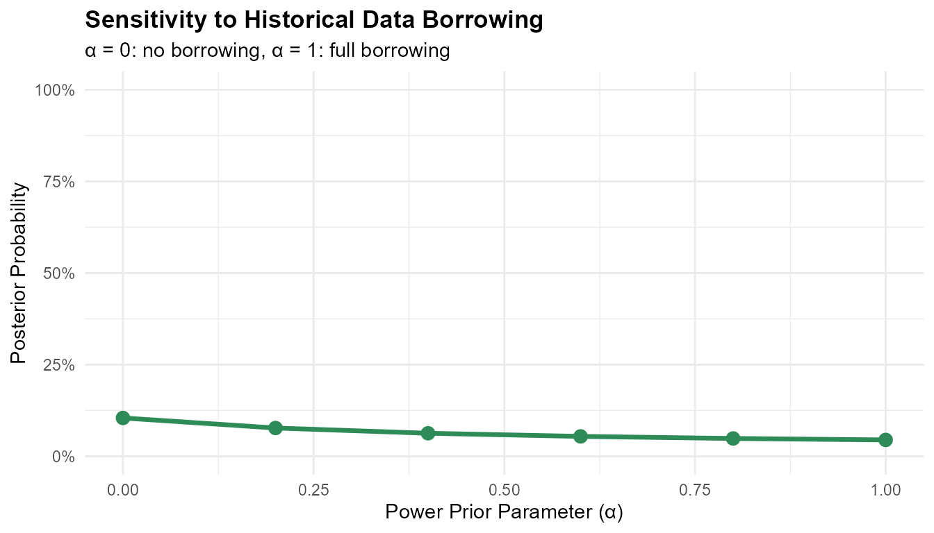

Sample Size and Power

Power Analysis Across Sample Sizes

# Evaluate optimal sample size for desired operating characteristics
sample_sizes <- seq(10, 50, by = 10)

oc_results_n <- do.call(rbind, lapply(sample_sizes, function(n) {
  result <- pGNGsinglecontinuous(
    nsim = 30,  # Reduced for vignette speed
    prob = 'posterior', design = 'controlled', prior = 'vague', CalcMethod = 'WS',
    theta.TV = 1.5, theta.MAV = 0.5, theta.NULL = NULL,
    nMC = NULL, gamma1 = 0.8, gamma2 = 0.3,
    n1 = n, n2 = n, m1 = NULL, m2 = NULL,
    kappa01 = NULL, kappa02 = NULL, nu01 = NULL, nu02 = NULL,
    mu01 = NULL, mu02 = NULL, sigma01 = NULL, sigma02 = NULL,
    mu1 = 5, mu2 = 3,  # Assume true effect of 2.0
    sigma1 = 2, sigma2 = 2,
    r = NULL, ne1 = NULL, ne2 = NULL, alpha01 = NULL, alpha02 = NULL,
    bar.ye1 = NULL, bar.ye2 = NULL, se1 = NULL, se2 = NULL,
    seed = 123
  )
  
  data.frame(
    sample_size = n,
    go_prob = result$Go,
    nogo_prob = result$NoGo,
    gray_prob = result$Gray
  )
}))

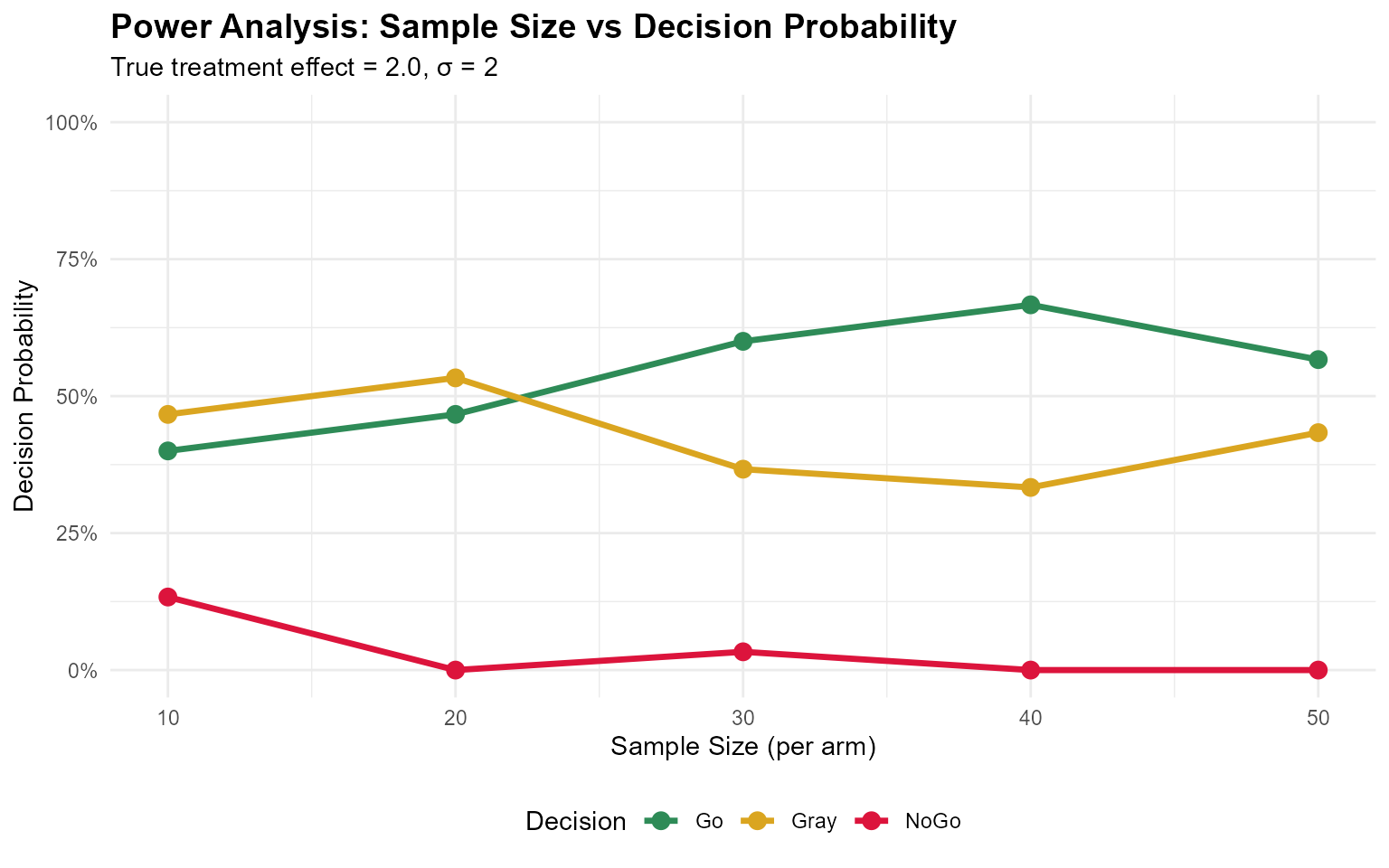
print(oc_results_n)
#>   sample_size   go_prob  nogo_prob gray_prob
#> 1          10 0.4000000 0.13333333 0.4666667
#> 2          20 0.4666667 0.00000000 0.5333333
#> 3          30 0.6000000 0.03333333 0.3666667
#> 4          40 0.6666667 0.00000000 0.3333333
#> 5          50 0.5666667 0.00000000 0.4333333

# Reshape for plotting
power_plot_data <- oc_results_n %>%
  pivot_longer(cols = c(go_prob, gray_prob, nogo_prob), 
               names_to = "decision", 
               values_to = "probability") %>%
  mutate(Decision = case_when(
    decision == "go_prob" ~ "Go",
    decision == "gray_prob" ~ "Gray",
    decision == "nogo_prob" ~ "NoGo"
  ))

ggplot(power_plot_data, aes(x = sample_size, y = probability, color = Decision)) +
  geom_line(linewidth = 1.2) +
  geom_point(size = 3) +
  scale_color_manual(values = c("Go" = "#2E8B57", "Gray" = "#DAA520", "NoGo" = "#DC143C")) +
  labs(
    title = "Power Analysis: Sample Size vs Decision Probability",
    x = "Sample Size (per arm)",
    y = "Decision Probability",
    subtitle = "True treatment effect = 2.0, σ = 2"
  ) +
  scale_y_continuous(limits = c(0, 1), labels = scales::percent) +
  theme_minimal() +
  theme(
    plot.title = element_text(face = "bold", size = 14),
    legend.position = "bottom"
  )

Practical Guidelines

Method Selection

NI (Numerical Integration) - Most accurate - Recommended for final analyses and regulatory submissions - Moderate computational time

WS (Welch-Satterthwaite) - Fast approximation - Good for exploratory analyses and simulations - Very close to NI results in most cases

MC (Monte Carlo) - Flexible but slowest - Use when other methods are not applicable - Requires careful selection of nMC (typically 10,000+)

Design Selection

1. Controlled: Standard two-arm trial with concurrent controls
2. Uncontrolled: Single-arm when ethical/practical constraints prevent randomization
3. External: When incorporating historical data can reduce sample size requirements

Threshold Selection

• θ_TV (Target Value): Clinically meaningful difference
• θ_MAV (Minimum Acceptable Value): Smallest worthwhile effect
• γ₁ (Go threshold): 0.7-0.9 depending on risk tolerance
• γ₂ (NoGo threshold): 0.2-0.4 for early stopping

Summary

This vignette demonstrated:

1. Basic probability calculations for continuous endpoints
2. Method comparison (NI, WS, MC)
3. Go/NoGo/Gray decision framework implementation
4. Operating characteristics evaluation
5. Prior specification (vague vs informative)
6. External control design with power priors
7. Sample size and power considerations

The BayesianQDM package provides flexible and rigorous tools for Bayesian decision-making in clinical trials with continuous endpoints.

References

For more details on the statistical methods, see:

• The main BayesianQDM vignette for framework overview
• Function documentation for parameter specifications
• The binary endpoints vignette for analysis of discrete outcomes