Bayesian Decision Making for Binary Endpoints

library(BayesianQDM)
library(dplyr)
#> 
#> Attaching package: 'dplyr'
#> The following objects are masked from 'package:stats':
#> 
#>     filter, lag
#> The following objects are masked from 'package:base':
#> 
#>     intersect, setdiff, setequal, union
library(tidyr)
library(ggplot2)

Introduction

The BayesianQDM package provides comprehensive methods for Bayesian quantitative decision-making in clinical trials with binary endpoints. This vignette demonstrates how to use the package for calculating posterior probabilities, posterior predictive probabilities, and Go/NoGo/Gray decision probabilities.

Basic Concepts

Decision Framework

The Bayesian decision-making framework categorizes trial outcomes into three zones:

• Go: Evidence suggests the treatment is effective (proceed to next phase)
• NoGo: Evidence suggests the treatment is not effective (stop development)
• Gray: Evidence is inconclusive (may need additional data)

Probability Types

Two types of probabilities can be calculated:

1. Posterior Probability: $P(\theta > \theta_0 | data)$ where $\theta$ is the treatment effect
2. Posterior Predictive Probability: $P(\text{future trial will show } \theta > \theta_0 | \text{current data})$

Basic Examples

Posterior Probability

# Calculate posterior probability for a controlled design
posterior_prob <- pPPsinglebinary(
  prob = 'posterior', 
  design = 'controlled', 
  theta0 = 0.15,
  n1 = 20, n2 = 20, y1 = 12, y2 = 8,
  a1 = 0.5, a2 = 0.5, b1 = 0.5, b2 = 0.5,
  m1 = NULL, m2 = NULL,
  ne1 = NULL, ne2 = NULL, ye1 = NULL, ye2 = NULL, ae1 = NULL, ae2 = NULL
)

cat("Posterior probability that treatment effect > 0.15:", round(posterior_prob, 4))
#> Posterior probability that treatment effect > 0.15: 0.3871

Posterior Predictive Probability

# Calculate posterior predictive probability
predictive_prob <- pPPsinglebinary(
  prob = 'predictive', 
  design = 'controlled', 
  theta0 = 0.15,
  n1 = 20, n2 = 20, y1 = 12, y2 = 8,
  a1 = 0.5, a2 = 0.5, b1 = 0.5, b2 = 0.5,
  m1 = 50, m2 = 50,
  ne1 = NULL, ne2 = NULL, ye1 = NULL, ye2 = NULL, ae1 = NULL, ae2 = NULL
)

cat("Predictive probability for future trial:", round(predictive_prob, 4))
#> Predictive probability for future trial: 0.4035

Go/NoGo/Gray Decision Probabilities

Basic Usage

# Calculate Go/NoGo/Gray probabilities
result <- pGNGsinglebinary(
  prob = 'posterior', 
  design = 'controlled',
  theta.TV = 0.3, theta.MAV = 0.1, theta.NULL = NULL,
  gamma1 = 0.8, gamma2 = 0.2,
  pi1 = c(0.3, 0.5, 0.7), 
  pi2 = rep(0.2, 3),
  n1 = 20, n2 = 20,
  a1 = 0.5, a2 = 0.5, b1 = 0.5, b2 = 0.5,
  z = NULL, m1 = NULL, m2 = NULL,
  ne1 = NULL, ne2 = NULL, ye1 = NULL, ye2 = NULL, ae1 = NULL, ae2 = NULL
)

print(result)
#>   pi1 pi2          Go      Gray       NoGo
#> 1 0.3 0.2 0.007803538 0.1821623 0.81003417
#> 2 0.5 0.2 0.192004138 0.5121603 0.29583556
#> 3 0.7 0.2 0.716236863 0.2583638 0.02539935

Operating Characteristics

Evaluating Across Scenarios

# Evaluate operating characteristics across different response rates
oc_results <- pGNGsinglebinary(
  prob = 'posterior', 
  design = 'controlled',
  theta.TV = 0.2, theta.MAV = 0.05, theta.NULL = NULL,
  gamma1 = 0.8, gamma2 = 0.2,
  pi1 = seq(0.2, 0.6, by = 0.1), 
  pi2 = rep(0.2, 5),
  n1 = 25, n2 = 25,
  a1 = 0.5, a2 = 0.5, b1 = 0.5, b2 = 0.5,
  z = NULL, m1 = NULL, m2 = NULL,
  ne1 = NULL, ne2 = NULL, ye1 = NULL, ye2 = NULL, ae1 = NULL, ae2 = NULL
)

print(oc_results)
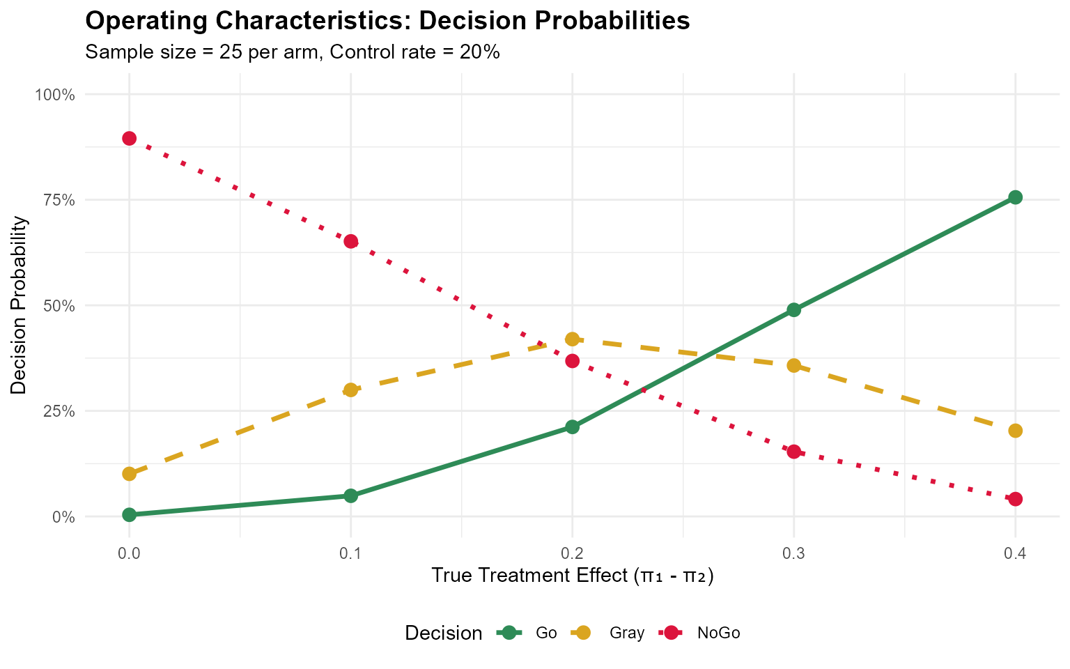
#>   pi1 pi2          Go      Gray       NoGo
#> 1 0.2 0.2 0.003871119 0.1008739 0.89525497
#> 2 0.3 0.2 0.048889816 0.2996013 0.65150893
#> 3 0.4 0.2 0.211943660 0.4198488 0.36820753
#> 4 0.5 0.2 0.489175480 0.3574133 0.15341120
#> 5 0.6 0.2 0.755770714 0.2030452 0.04118413

Visualizing Decision Probabilities

# Reshape data for plotting
plot_data <- oc_results %>%
  select(pi1, pi2, Go, NoGo, Gray) %>%
  pivot_longer(cols = c(Go, NoGo, Gray), 
               names_to = "Decision", 
               values_to = "Probability") %>%
  mutate(TreatmentEffect = pi1 - pi2)

ggplot(plot_data, aes(x = TreatmentEffect, y = Probability, color = Decision, linetype = Decision)) +
  geom_line(linewidth = 1.2) +
  geom_point(size = 3) +
  scale_color_manual(values = c("Go" = "#2E8B57", "Gray" = "#DAA520", "NoGo" = "#DC143C")) +
  scale_linetype_manual(values = c("Go" = "solid", "Gray" = "dashed", "NoGo" = "dotted")) +
  labs(
    title = "Operating Characteristics: Decision Probabilities",
    subtitle = "Sample size = 25 per arm, Control rate = 20%",
    x = "True Treatment Effect (π₁ - π₂)",
    y = "Decision Probability"
  ) +
  scale_y_continuous(limits = c(0, 1), labels = scales::percent) +
  theme_minimal() +
  theme(
    plot.title = element_text(face = "bold", size = 14),
    legend.position = "bottom"
  )

Study Designs

Controlled Design

Standard two-arm randomized controlled trial.

result_controlled <- pPPsinglebinary(
  prob = 'posterior', 
  design = 'controlled', 
  theta0 = 0.15,
  n1 = 20, n2 = 20, y1 = 12, y2 = 8,
  a1 = 0.5, a2 = 0.5, b1 = 0.5, b2 = 0.5,
  m1 = NULL, m2 = NULL,
  ne1 = NULL, ne2 = NULL, ye1 = NULL, ye2 = NULL, ae1 = NULL, ae2 = NULL
)

cat("Controlled design posterior probability:", round(result_controlled, 4))
#> Controlled design posterior probability: 0.3871

Uncontrolled Design

Single-arm study with historical control.

result_uncontrolled <- pPPsinglebinary(
  prob = 'posterior', 
  design = 'uncontrolled', 
  theta0 = 0.15,
  n1 = 20, n2 = 20, y1 = 12, y2 = 4,  # y2 represents historical control response
  a1 = 0.5, a2 = 0.5, b1 = 0.5, b2 = 0.5,
  m1 = NULL, m2 = NULL,
  ne1 = NULL, ne2 = NULL, ye1 = NULL, ye2 = NULL, ae1 = NULL, ae2 = NULL
)

cat("Uncontrolled design posterior probability:", round(result_uncontrolled, 4))
#> Uncontrolled design posterior probability: 0.0515

External Control Design

Incorporating historical data through power priors.

# External control with 50% borrowing
result_external <- pPPsinglebinary(
  prob = 'posterior', 
  design = 'external', 
  theta0 = 0.15,
  n1 = 20, n2 = 20, y1 = 12, y2 = 8,
  a1 = 0.5, a2 = 0.5, b1 = 0.5, b2 = 0.5,
  m1 = NULL, m2 = NULL,
  ne1 = 15, ne2 = 25, ye1 = 9, ye2 = 10, ae1 = 0.5, ae2 = 0.5
)

cat("External control posterior probability:", round(result_external, 4))
#> External control posterior probability: 0.3579

Sensitivity to Power Prior Parameter

# Evaluate sensitivity to borrowing parameter (varying both ae1 and ae2)
alpha_values <- seq(0, 1, by = 0.2)

borrowing_results <- data.frame(
  alpha = alpha_values,
  probability = sapply(alpha_values, function(a) {
    pPPsinglebinary(
      prob = 'posterior', design = 'external', theta0 = 0.15,
      n1 = 20, n2 = 20, y1 = 12, y2 = 8,
      a1 = 0.5, a2 = 0.5, b1 = 0.5, b2 = 0.5,
      m1 = NULL, m2 = NULL,
      ne1 = 15, ne2 = 25, ye1 = 9, ye2 = 10, ae1 = a, ae2 = a
    )
  })
)

print(borrowing_results)
#>   alpha probability
#> 1   0.0   0.3870664
#> 2   0.2   0.3743445
#> 3   0.4   0.3630836
#> 4   0.6   0.3528975
#> 5   0.8   0.3435474
#> 6   1.0   0.3348736

ggplot(borrowing_results, aes(x = alpha, y = probability)) +
  geom_line(linewidth = 1.2, color = '#2E8B57') +
  geom_point(size = 3, color = '#2E8B57') +
  labs(
    title = "Sensitivity to Historical Data Borrowing",
    x = "Power Prior Parameter (α)",
    y = "Posterior Probability",
    subtitle = "α = 0: no borrowing, α = 1: full borrowing"
  ) +
  scale_y_continuous(limits = c(0, 1), labels = scales::percent) +
  theme_minimal() +
  theme(plot.title = element_text(face = "bold"))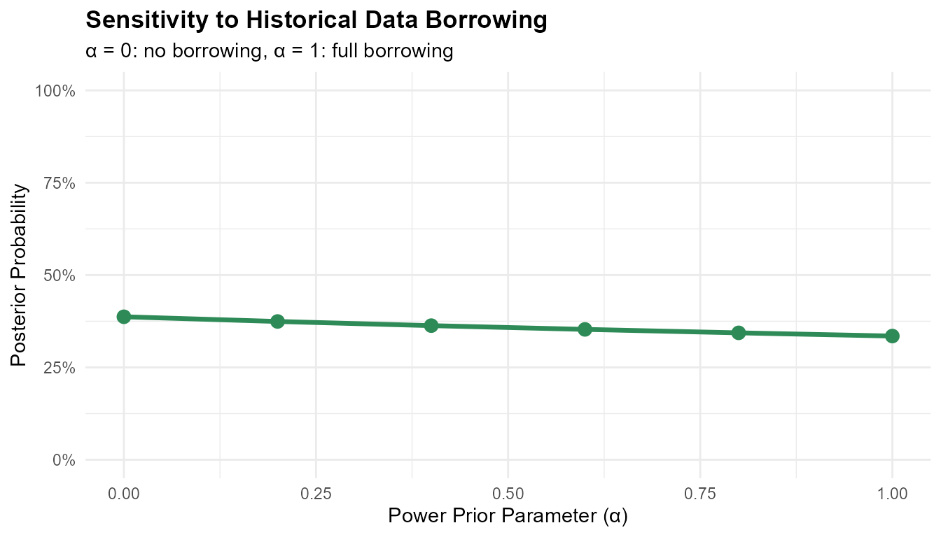

Sample Size Considerations

Power Analysis

# Evaluate power across different sample sizes
sample_sizes <- seq(10, 50, by = 10)

power_results <- data.frame(
  n = sample_sizes,
  go_prob = sapply(sample_sizes, function(n) {
    result <- pGNGsinglebinary(
      prob = 'posterior', design = 'controlled',
      theta.TV = 0.2, theta.MAV = 0.05, theta.NULL = NULL,
      gamma1 = 0.8, gamma2 = 0.2,
      pi1 = 0.5, pi2 = 0.3,  # Assume true effect of 0.2
      n1 = n, n2 = n,
      a1 = 0.5, a2 = 0.5, b1 = 0.5, b2 = 0.5,
      z = NULL, m1 = NULL, m2 = NULL,
      ne1 = NULL, ne2 = NULL, ye1 = NULL, ye2 = NULL, ae1 = NULL, ae2 = NULL
    )
    result$Go[1]
  })
)

print(power_results)
#>    n   go_prob
#> 1 10 0.2447746
#> 2 20 0.2058666
#> 3 30 0.1762386
#> 4 40 0.2079638
#> 5 50 0.1775540

ggplot(power_results, aes(x = n, y = go_prob)) +
  geom_line(linewidth = 1.2, color = '#2E8B57') +
  geom_point(size = 3, color = '#2E8B57') +
  geom_hline(yintercept = 0.8, linetype = "dashed", color = "red") +
  annotate("text", x = 45, y = 0.85, label = "Target: 80%", color = "red") +
  labs(
    title = "Power Analysis: Sample Size vs Go Probability",
    x = "Sample Size (per arm)",
    y = "Go Probability",
    subtitle = "True treatment effect = 20%"
  ) +
  scale_y_continuous(limits = c(0, 1), labels = scales::percent) +
  theme_minimal() +
  theme(plot.title = element_text(face = "bold"))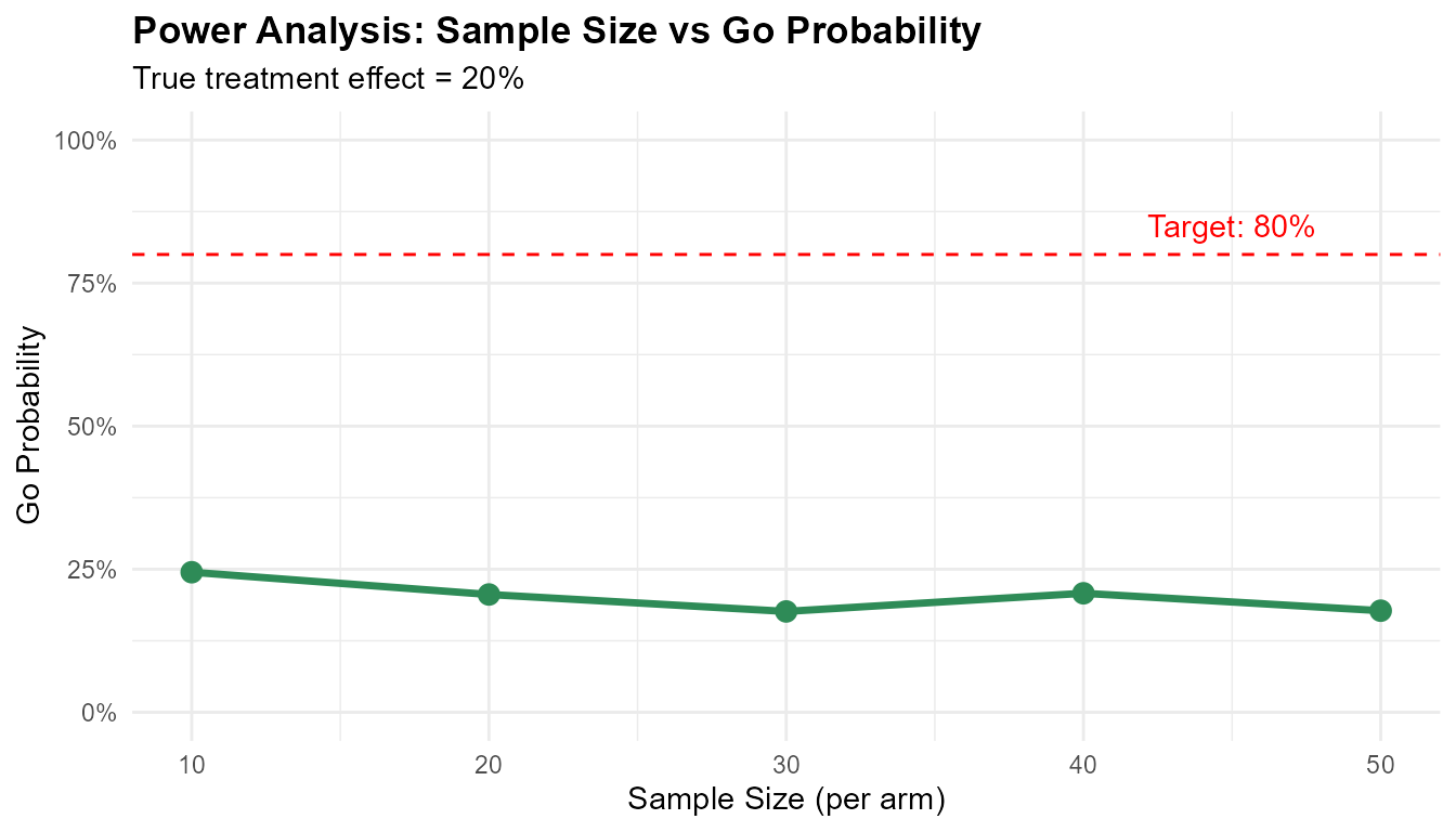

Practical Guidelines

Threshold Selection

When designing a trial, consider:

• θ_TV (Target Value): Set based on clinically meaningful difference
• θ_MAV (Minimum Acceptable Value): Set based on smallest worthwhile effect
• γ₁ (Go threshold): Typically 0.8-0.9 for high confidence
• γ₂ (NoGo threshold): Typically 0.2-0.3 for early stopping

Prior Selection

• Weakly informative: Beta(0.5, 0.5) - Jeffreys prior
• Uniform: Beta(1, 1) - uniform prior
• Informative: Beta(a, b) based on historical data or expert opinion

Design Selection

1. Controlled: Standard two-arm trial (most common)
2. Uncontrolled: Single-arm when historical control is well-established
3. External: When incorporating historical data via power priors

Summary

This vignette demonstrated:

1. Basic probability calculations for binary endpoints
2. Go/NoGo/Gray decision framework with customizable thresholds
3. Operating characteristics evaluation across scenarios
4. External control design with power priors
5. Sample size considerations for trial planning

The BayesianQDM package provides flexible tools for evidence-based decision making in clinical trials with binary endpoints.

References

For more details on the statistical methods, see:

• The main BayesianQDM vignette for framework overview
• Function documentation for parameter specifications
• The continuous endpoints vignette for analysis of continuous outcomes