library(CorOncoEndpoints)
set.seed(123)
Overview
This vignette demonstrates advanced usage of the
CorOncoEndpoints package, including:
- Working with the three-endpoint framework (OS + PFS + Response)
- Understanding implied correlations
- Sensitivity analyses
- Complex simulation studies
- Visualization techniques
The Three-Endpoint Framework
When generating all three endpoints simultaneously, understanding the correlation structure is crucial.
Key Insight
When you specify: - p: Response probability -
hazard_OS: OS hazard rate - hazard_PFS: PFS
hazard rate
- rho_tte_resp: Correlation between OS and
Response
The correlation between PFS and Response is automatically determined by the model structure (Fleischer model).
Example: Understanding Implied Correlations
# Parameters
p <- 0.4
hazard_OS <- 0.05
hazard_PFS <- 0.08
rho_OS_Response <- 0.3

# Calculate implied PFS-Response correlation
rho_PFS_Response <- CorResponsePFS(
  p = p,
  hazard_OS = hazard_OS,
  hazard_PFS = hazard_PFS,
  rho_OS_Response = rho_OS_Response,
  copula = "Clayton"
)

cat("Specified OS-Response correlation:", rho_OS_Response, "\n")
#> Specified OS-Response correlation: 0.3
cat("Implied PFS-Response correlation:", round(rho_PFS_Response, 3), "\n")
#> Implied PFS-Response correlation: 0.243

# Verify with simulation
data <- rOncoEndpoints(
  nsim = 1000,
  n = 200,
  p = p,
  hazard_OS = hazard_OS,
  hazard_PFS = hazard_PFS,
  rho_tte_resp = rho_OS_Response,
  copula = "Clayton"
)

# Empirical correlations
sim1 <- subset(data, simID == 1)
cat("\nEmpirical OS-Response correlation:",
    round(cor(sim1$OS, sim1$Response), 3), "\n")
#>
#> Empirical OS-Response correlation: 0.266
cat("Empirical PFS-Response correlation:",
    round(cor(sim1$PFS, sim1$Response), 3), "\n")
#> Empirical PFS-Response correlation: 0.32
Correlation Bounds in Three-Endpoint Framework
The feasible range for PFS-Response correlation depends on both the response probability AND the hazard rates:
# General TTE-Response bounds (depends only on p)
general_bounds <- CorBoundResponseTTE(p = 0.4)
cat("General TTE-Response bounds:",
    round(general_bounds[1], 3), "to", round(general_bounds[2], 3), "\n")
#> General TTE-Response bounds: -0.626 to 0.748

# PFS-Response bounds in OS-PFS-Response framework
pfs_bounds <- CorBoundResponsePFS(
  p = 0.4,
  hazard_OS = 0.05,
  hazard_PFS = 0.08
)
cat("PFS-Response bounds (3-endpoint):",
    round(pfs_bounds[1], 3), "to", round(pfs_bounds[2], 3), "\n")
#> PFS-Response bounds (3-endpoint): -0.539 to 0.576
Notice that the PFS-specific bounds are typically narrower.
Sensitivity Analysis
Effect of Hazard Ratio on Correlations
# Fixed parameters
p <- 0.5
hazard_OS <- 0.04
rho_OS <- 0.3

# Varying hazard ratios
hazard_ratios <- seq(1.5, 3.0, by = 0.1)
hazard_PFS_vec <- hazard_OS * hazard_ratios

# Calculate implied PFS-Response correlations
rho_PFS_vec <- sapply(hazard_PFS_vec, function(h_pfs) {
  CorResponsePFS(p, hazard_OS, h_pfs, rho_OS, copula = "Clayton")
})

# Plot
plot(hazard_ratios, rho_PFS_vec, type = "b",
     xlab = "Hazard Ratio (PFS/OS)",
     ylab = "Correlation",
     main = "Effect of Hazard Ratio on PFS-Response Correlation",
     ylim = range(c(rho_PFS_vec, rho_OS)))
abline(h = rho_OS, lty = 2, col = "red", lwd = 2)
legend("topright",
       legend = c("PFS-Response correlation",
                  paste0("OS-Response correlation (", rho_OS, ")")),
       lty = c(1, 2), col = c("black", "red"), pch = c(1, NA), lwd = c(1, 2))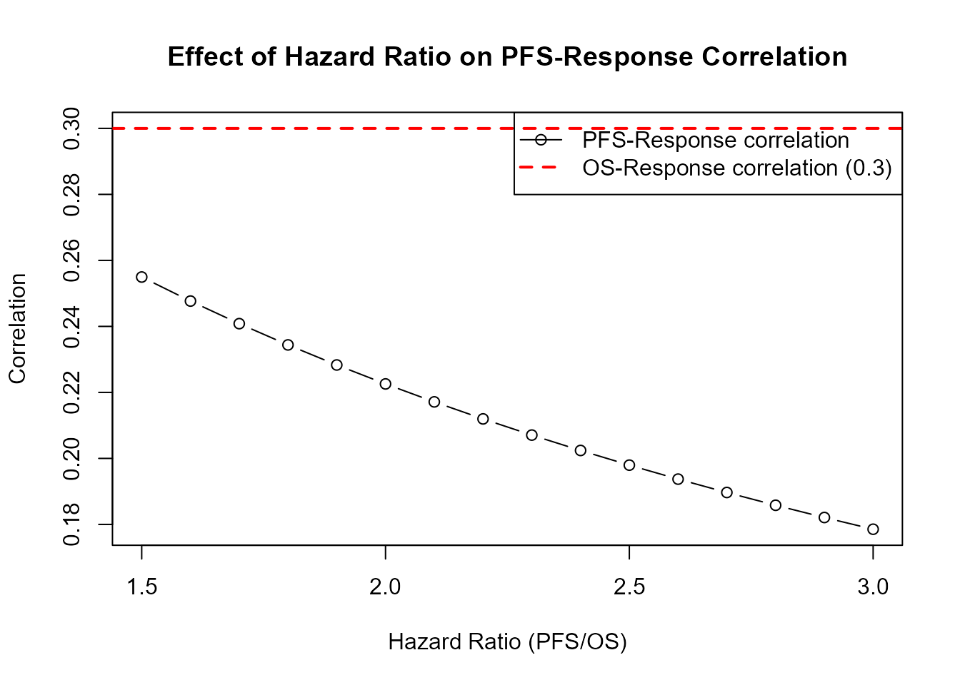
Interpretation: As the hazard ratio increases (PFS becomes shorter relative to OS), the PFS-Response correlation decreases.
Effect of Response Probability
# Varying response probabilities
p_vec <- seq(0.2, 0.8, by = 0.05)

# Calculate bounds for each p
bounds_matrix <- sapply(p_vec, CorBoundResponseTTE)

# Plot
plot(p_vec, bounds_matrix[2, ], type = "l", col = "blue", lwd = 2,
     ylim = range(bounds_matrix), xlab = "Response Probability (p)",
     ylab = "Correlation Bound",
     main = "Feasible Correlation Range by Response Probability")
lines(p_vec, bounds_matrix[1, ], col = "red", lwd = 2)
abline(h = 0, lty = 2, col = "gray")
legend("topright", legend = c("Upper Bound", "Lower Bound"),
       col = c("blue", "red"), lty = 1, lwd = 2)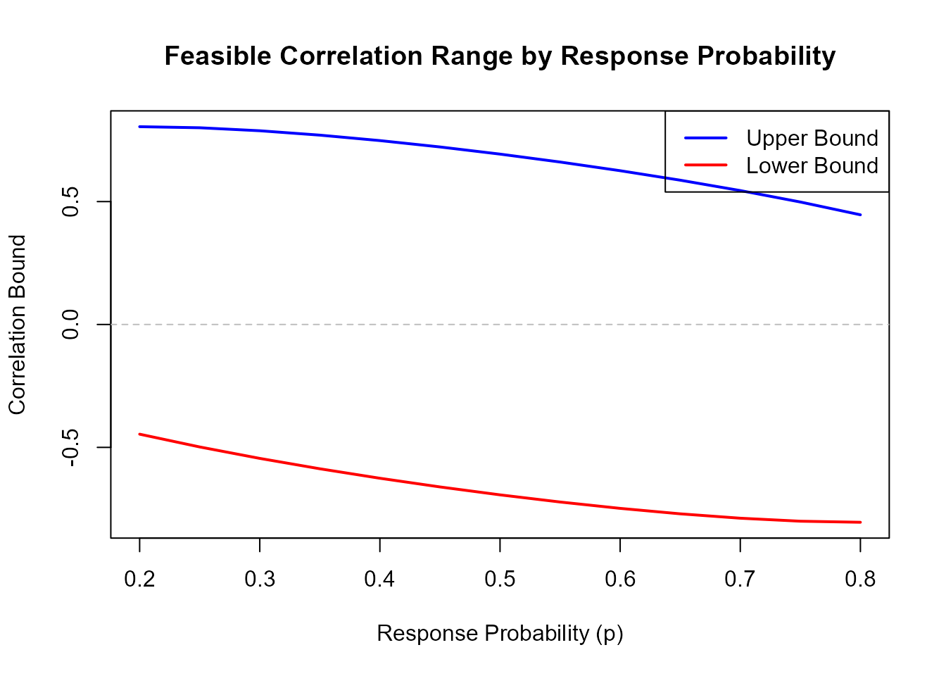
Complex Simulation Studies
Multi-Arm Trial Simulation
# Three-arm trial: Placebo, Low Dose, High Dose
data_multi <- rOncoEndpoints(
  nsim = 500,
  group = c("Placebo", "Low Dose", "High Dose"),
  n = c(100, 100, 100),
  p = c(0.2, 0.35, 0.5),
  hazard_OS = c(0.08, 0.06, 0.04),
  hazard_PFS = c(0.12, 0.10, 0.08),
  rho_tte_resp = c(0.2, 0.3, 0.4),
  copula = "Frank"
)

# Validate results
validation_multi <- CheckSimResults(
  dataset = data_multi,
  p = c(Placebo = 0.2, `Low Dose` = 0.35, `High Dose` = 0.5),
  hazard_OS = c(Placebo = 0.08, `Low Dose` = 0.06, `High Dose` = 0.04),
  hazard_PFS = c(Placebo = 0.12, `Low Dose` = 0.10, `High Dose` = 0.08),
  rho_tte_resp = c(Placebo = 0.2, `Low Dose` = 0.3, `High Dose` = 0.4),
  copula = "Frank"
)

# Show median survival times
medians <- validation_multi[validation_multi$Endpoint %in%
                             c("OS_Median", "PFS_Median"),
                             c("Group", "Endpoint", "Empirical", "Theoretical")]
print(medians, n = Inf)
#> # A tibble: 6 × 4
#>   Group     Endpoint   Empirical Theoretical
#>   <chr>     <chr>          <dbl>       <dbl>
#> 1 Placebo   OS_Median       8.68        8.66
#> 2 Placebo   PFS_Median      5.80        5.78
#> 3 Low Dose  OS_Median      11.6        11.6
#> 4 Low Dose  PFS_Median      6.95        6.93
#> 5 High Dose OS_Median      17.2        17.3
#> 6 High Dose PFS_Median      8.68        8.66
Time-Varying Sample Size
# Simulate different sample sizes per simulation
# (Useful for adaptive designs)
n_per_sim <- sample(80:120, size = 100, replace = TRUE)

# Generate data with varying n
# Note: rOncoEndpoints requires fixed n per group, so we'll
# generate multiple datasets

results_list <- lapply(1:10, function(i) {
  rOncoEndpoints(
    nsim = 1,
    n = n_per_sim[i],
    p = 0.4,
    hazard_OS = 0.05,
    rho_tte_resp = 0.3,
    copula = "Clayton"
  )
})

# Combine results
data_varying <- do.call(rbind, results_list)
table(data_varying$simID)
#>
#>   1
#> 967
Copula Parameter Exploration
Relationship Between Correlation and Theta
# For different correlations, calculate copula parameters
rho_vec <- seq(0.1, 0.6, by = 0.05)
p <- 0.4

theta_clayton <- sapply(rho_vec, function(r) {
  CopulaParamResponseTTE(p, r, "Clayton")
})

theta_frank <- sapply(rho_vec, function(r) {
  CopulaParamResponseTTE(p, r, "Frank")
})

# Plot
par(mfrow = c(1, 2))
plot(rho_vec, theta_clayton, type = "b", col = "blue",
     xlab = "Correlation", ylab = "Theta",
     main = "Clayton Copula: Correlation vs Theta")

plot(rho_vec, theta_frank, type = "b", col = "red",
     xlab = "Correlation", ylab = "Theta",
     main = "Frank Copula: Correlation vs Theta")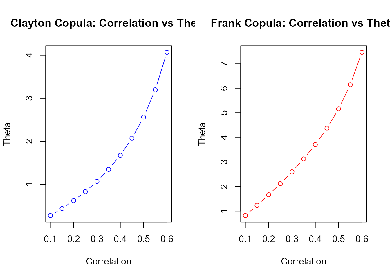
Practical Applications
Application 1: Endpoint Selection Study
Compare power for different endpoint choices:
# Scenario: Which endpoint provides better power?
# Generate data for multiple scenarios

# OS only
data_os <- rOncoEndpoints(
  nsim = 500,
  group = c("Treatment", "Control"),
  n = c(150, 150),
  hazard_OS = c(0.05, 0.07)
)

# Response only
data_resp <- rOncoEndpoints(
  nsim = 500,
  group = c("Treatment", "Control"),
  n = c(150, 150),
  p = c(0.4, 0.3)
)

# OS + Response
data_both <- rOncoEndpoints(
  nsim = 500,
  group = c("Treatment", "Control"),
  n = c(150, 150),
  p = c(0.4, 0.3),
  hazard_OS = c(0.05, 0.07),
  rho_tte_resp = c(0.3, 0.2),
  copula = "Clayton"
)

# Calculate effect sizes for each endpoint type
# (Analysis code would go here)
Application 2: Correlation Impact Study
How does the correlation structure affect trial outcomes?
# Generate data with different correlation structures
correlations <- c(0.1, 0.3, 0.5)

data_list <- lapply(correlations, function(rho) {
  rOncoEndpoints(
    nsim = 200,
    group = "Treatment",
    n = 100,
    p = 0.4,
    hazard_OS = 0.05,
    rho_tte_resp = rho,
    copula = "Clayton"
  )
})

# Compare variability in endpoints across correlations
variances <- sapply(data_list, function(d) {
  c(
    var_OS = var(d$OS),
    var_Response = var(d$Response)
  )
})

colnames(variances) <- paste("rho =", correlations)
print(round(variances, 3))
#>              rho = 0.1 rho = 0.3 rho = 0.5
#> var_OS         396.565   399.321   391.955
#> var_Response     0.241     0.240     0.240
Application 3: Model Misspecification Study
What happens if we assume independence when data are correlated?
# Generate correlated data
data_corr <- rOncoEndpoints(
  nsim = 1000,
  n = 200,
  p = 0.4,
  hazard_OS = 0.05,
  rho_tte_resp = 0.4,
  copula = "Clayton"
)

# Analyze assuming independence vs accounting for correlation
# (Statistical analysis code would go here)

# Calculate empirical correlation
sim1_corr <- subset(data_corr, simID == 1)
cat("True correlation:", 0.4, "\n")
#> True correlation: 0.4
cat("Empirical correlation:",
    round(cor(sim1_corr$OS, sim1_corr$Response), 3), "\n")
#> Empirical correlation: 0.433
Visualization Techniques
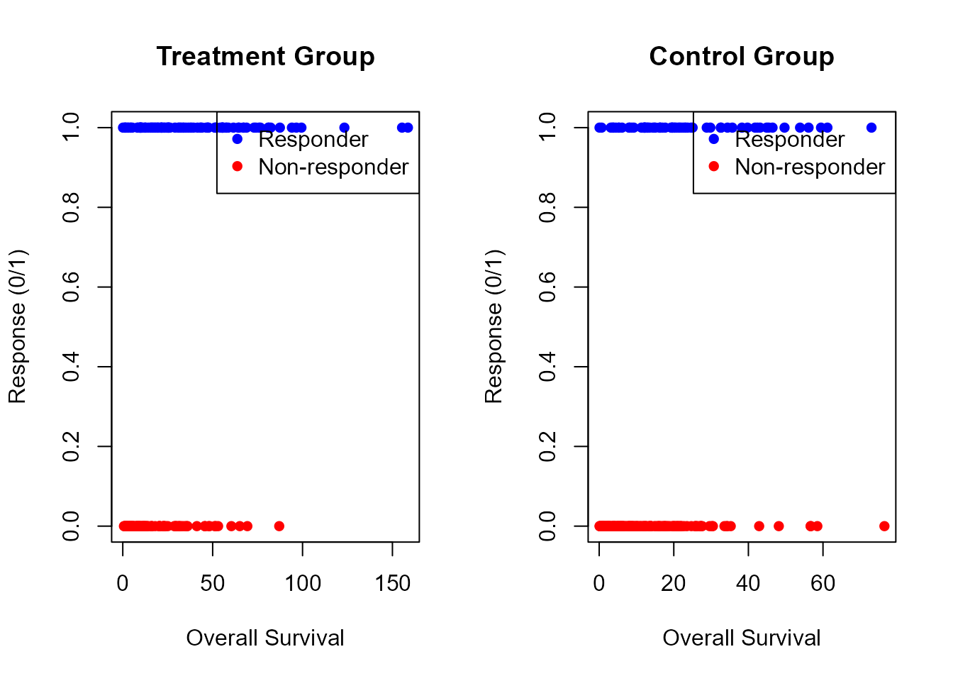
Correlation Structure Visualization
# Generate data
data_viz <- rOncoEndpoints(
  nsim = 1,
  group = c("Treatment", "Control"),
  n = c(200, 200),
  p = c(0.5, 0.3),
  hazard_OS = c(0.04, 0.06),
  hazard_PFS = c(0.08, 0.10),
  rho_tte_resp = c(0.4, 0.2),
  copula = "Frank"
)

# Scatter plot: OS vs Response by group
par(mfrow = c(1, 2))
for (grp in c("Treatment", "Control")) {
  d <- subset(data_viz, Group == grp)
  plot(d$OS, d$Response,
       main = paste(grp, "Group"),
       xlab = "Overall Survival",
       ylab = "Response (0/1)",
       pch = 16, col = ifelse(d$Response == 1, "blue", "red"))
  legend("topright",
         legend = c("Responder", "Non-responder"),
         col = c("blue", "red"), pch = 16)
}
Best Practices
-
Always validate: Use
CheckSimResults()to ensure simulations match theory -
Check bounds: Use
CorBoundResponseTTE()before specifying correlations - Understand three-endpoint model: Remember that PFS-Response correlation is derived
- Choose appropriate copula: Clayton for positive correlations only, Frank for flexibility
- Use adequate simulations: At least 1000 simulations for stable results
- Document assumptions: Clearly state hazard rates, correlations, and copula choices
Summary
This vignette covered:
- The three-endpoint framework and implied correlations
- Sensitivity analyses for key parameters
- Complex simulation study designs
- Copula parameter exploration
- Practical applications
- Visualization techniques
For theoretical details, see the “Theoretical Background” vignette.