
Group-sequential design with correlated PFS and OS under the Fleischer model
Source:vignettes/correlated-pfs-os-gsd.Rmd
correlated-pfs-os-gsd.RmdOverview
Many confirmatory oncology trials test progression-free survival (PFS) as the primary endpoint and overall survival (OS) as a key secondary endpoint, with the two endpoints tested in a fixed sequence to control the family-wise error rate. A PFS event is a progression or a death, so a death before progression is an event for both endpoints, and the OS time is never shorter than the PFS time. The two endpoints are therefore positively correlated, and that correlation is needed to characterize the operating characteristics of the sequential procedure.
This vignette simulates such a design with the simulation trio
simdata_fast, analysis_fast, and
simsummary_fast. It generates correlated PFS and OS times
from the Fleischer maximal-independence model, runs an event-driven
group-sequential design with one futility analysis followed by two
efficacy analyses, evaluates the power of each endpoint under the
alternative, and estimates the correlation of the standardized log-rank
statistics Corr(Z_PFS, Z_OS). This correlation is the input
that a closed-form evaluation of the sequential procedure would need,
and the simulation gives the operating characteristics of the procedure
directly.
The Fleischer model
For a subject in group g the Fleischer
maximal-independence model (Fleischer, Gaschler-Markefski, and Bluhmki,
2009) takes an independent time-to-progression
TTP ~ Exp(lam1) and an overall survival time
OS ~ Exp(lam2), and sets
PFS = min(TTP, OS), OS = OS.Since TTP and OS are independent
exponentials, PFS is exponential with hazard
Lambda = lam1 + lam2. Given the medians of PFS and OS, the
OS hazard is lam2 = log(2) / median_OS and the PFS hazard
is Lambda = log(2) / median_PFS, so the implied TTP hazard
is lam1 = Lambda - lam2, which must be positive (median OS
longer than median PFS in each group). The dependence between the two
endpoints is induced entirely through the shared OS
component.
The design
The trial is event-driven with three synchronized analyses indexed by cumulative PFS event counts. The first analysis is a non-binding futility look on PFS; the second and third are the efficacy interim and the efficacy final. PFS is the primary endpoint and OS is the key secondary endpoint, and the two are tested in the order PFS then OS: OS is declared significant only if PFS has already been declared significant at the same or an earlier look. The analyses are timed by PFS events, and the OS analysis at each look reuses the same calendar cutoff as the PFS analysis. The PFS efficacy boundary uses an O’Brien-Fleming Lan-DeMets alpha-spending function and the OS efficacy boundary uses a Pocock-type Lan-DeMets spending function, each at a one-sided level of 0.025 and each spent over the two efficacy looks. All tests are the ordinary unweighted log-rank test, one-sided in the direction of treatment benefit.
Design parameters
nsim <- 5000
seed <- 20260611

# Per-group sample sizes (group 1 = control, group 2 = treatment)
n_control <- 300
n_treat   <- 300
r_alloc   <- n_treat / n_control          # allocation ratio treatment:control

# Piecewise-uniform accrual: 20 per month, then 40 per month (600 enrolled by month 18)
a_time <- c(0, 6)
a_rate <- c(20, 40)

# Median PFS and OS by group, in months
mst_PFS_C <- 6
mst_PFS_T <- 9
mst_OS_C  <- 14
mst_OS_T  <- 18

# Exponential hazards implied by the medians
lam_PFS_C <- log(2) / mst_PFS_C
lam_PFS_T <- log(2) / mst_PFS_T
lam_OS_C  <- log(2) / mst_OS_C
lam_OS_T  <- log(2) / mst_OS_T

# Fleischer maximal-independence: PFS hazard = TTP hazard + OS hazard,
# so the latent TTP hazard is the PFS hazard minus the OS hazard.
lam_TTP_C <- lam_PFS_C - lam_OS_C
lam_TTP_T <- lam_PFS_T - lam_OS_T
stopifnot(lam_TTP_C > 0, lam_TTP_T > 0)

# Non-informative exponential dropout, 10 percent per year on the month scale
eta <- -log(1 - 0.10) / 12

# Event-driven looks (cumulative PFS event counts):
#   look 1 = futility, look 2 = efficacy interim, look 3 = efficacy final
d_PFS <- c(200, 300, 400)
L <- length(d_PFS)

# One-sided overall significance level
alpha_total <- 0.025

c(HR_PFS = lam_PFS_T / lam_PFS_C, HR_OS = lam_OS_T / lam_OS_C)
#>    HR_PFS     HR_OS
#> 0.6666667 0.7777778
The PFS hazard ratio is the stronger effect and the OS hazard ratio is more modest, which is the usual pattern when a treatment delays progression more than it extends survival.
Data generation
A single simdata_fast call generates the two correlated
endpoints directly from the illness-death structure. The intermediate
event (progression) has hazard h01 = lam_TTP and the
terminal event (death) has hazard h02 = lam_OS; the
post-progression death hazard is left at its default, equal to
h02, which reproduces the maximal-independence model
described above. The first endpoint e1 is PFS and the
terminal endpoint e2 is OS. The dropout time is shared
between the two endpoints, so a subject who drops out is censored for
both PFS and OS at the same time.
# A single call returns both correlated endpoints. e1 is PFS (the state-0 exit:
# progression or death), e2 is OS (the terminal event), and dropout_time is the
# shared non-informative dropout. The observed columns e1_tte / e1_event and
# e2_tte / e2_event are each already censored at the shared dropout time.
df <- simdata_fast(
  nsim       = nsim,
  n          = c(n_control, n_treat),
  a.time     = a_time,
  a.rate     = a_rate,
  h01.hazard = list(lam_TTP_C, lam_TTP_T),
  h02.hazard = list(lam_OS_C, lam_OS_T),
  d.hazard   = eta,
  seed       = seed
)

# Single-endpoint view of PFS (k = 1) or OS (k = 2), in the columns that
# analysis_fast() reads.
ep <- function(d, k) {
  data.frame(
    sim          = d$sim,
    group        = d$group,
    accrual_time = d$accrual_time,
    tte          = d[[paste0("e", k, "_tte")]],
    event        = d[[paste0("e", k, "_event")]]
  )
}
pfs_dat <- ep(df, 1)
os_dat  <- ep(df, 2)
Primary endpoint analysis (PFS)
PFS is analyzed at the three event-driven looks.
cutoff_fast returns, for every simulated trial, the
calendar time of the d_PFS[l]-th PFS event, which is the
analysis time of look l. It counts the events in the PFS
columns e1_tte and e1_event of the
illness-death data. These cutoffs are exactly the analysis times of the
design, and both endpoints are analyzed at them through the
cutoff.looks argument of analysis_fast.
# Per-simulation calendar cutoffs A_l (rows = simulation, columns = look),
# triggered by the PFS events.
A_mat <- cutoff_fast(df, event.looks = d_PFS,
                     tte.col = "e1_tte", event.col = "e1_event")

pfs_res <- analysis_fast(
  pfs_dat,
  control      = 1,
  cutoff.looks = A_mat,
  stat         = "logrank",
  side         = 1
)

# With this sample size and these event targets the looks are reached in
# essentially every simulation; warn if any target is not reached.
if (!all(pfs_res$reached)) {
  warning("Some PFS event targets were not reached; increase n or lower d_PFS.")
}

# Standardized PFS log-rank statistics (natural sign: benefit is negative)
Z_PFS <- matrix(pfs_res$logrank.z, nrow = nsim, ncol = L, byrow = TRUE)
The same analysis is obtained with event.looks = d_PFS,
which determines the cutoffs and analyzes PFS in one call; computing the
cutoffs separately lets the OS analysis reuse them.
Key secondary endpoint analysis (OS)
OS is analyzed at the same per-simulation cutoffs A_l.
At each look the OS times are administratively censored at
A_l, which reproduces the design rule that the OS analysis
at a look uses the PFS-driven analysis time.
os_res <- analysis_fast(
  os_dat,
  control      = 1,
  cutoff.looks = A_mat,
  stat         = "logrank",
  side         = 1
)

# Standardized OS log-rank statistics
Z_OS <- matrix(os_res$logrank.z, nrow = nsim, ncol = L, byrow = TRUE)
The mean PFS and OS event counts at each look summarize the information available to each endpoint. PFS reaches its event targets by construction, while OS, being the slower endpoint, accrues far fewer events at the same analysis times.
d_PFS_emp <- colMeans(matrix(pfs_res$n.event, nrow = nsim, ncol = L, byrow = TRUE))
d_OS_emp  <- colMeans(matrix(os_res$n.event,  nrow = nsim, ncol = L, byrow = TRUE))
A_mean    <- unname(colMeans(A_mat))

data.frame(
  look          = seq_len(L),
  d_PFS_target  = d_PFS,
  d_PFS_mean    = round(d_PFS_emp),
  d_OS_mean     = round(d_OS_emp),
  cutoff_months = round(A_mean, 1)
)
#>   look d_PFS_target d_PFS_mean d_OS_mean cutoff_months
#> 1    1          200        200       112          15.3
#> 2    2          300        300       175          19.0
#> 3    3          400        400       250          24.0
Efficacy and futility boundaries
Efficacy is assessed at the two later looks only. Two-look Lan-DeMets
alpha-spending boundaries are computed with gsDesign at the
information fractions implied by the event counts: the PFS information
fractions are the exact event-target ratios, and the OS information
fractions use the mean OS event counts. gsDesign reports
its boundaries on the convention that a positive Z favors the treatment,
so they are negated to match the natural sign of logrank.z,
where treatment benefit is a negative value. The first look carries a
non-binding futility rule on PFS, expressed as a threshold on the
standardized statistic.
The OS information fractions are planning values: they come from the mean OS event counts simulated under the alternative hypothesis, whereas a trial would use the observed counts at each analysis. This vignette evaluates power under the alternative only; the family-wise error rate of the hierarchical procedure would be checked by a further simulation under the null hypothesis for both endpoints (equal transition hazards in the two groups).
timing_PFS_eff <- c(d_PFS[2] / d_PFS[3], 1)
timing_OS_eff  <- c(d_OS_emp[2] / d_OS_emp[3], 1)

gs_PFS <- gsDesign::gsDesign(
  k = 2, test.type = 1, alpha = alpha_total,
  timing = timing_PFS_eff, sfu = gsDesign::sfLDOF
)
gs_OS <- gsDesign::gsDesign(
  k = 2, test.type = 1, alpha = alpha_total,
  timing = timing_OS_eff, sfu = gsDesign::sfLDPocock
)

b_PFS <- gs_PFS$upper$bound      # positive z-boundaries (interim, final)
b_OS  <- gs_OS$upper$bound

# Efficacy boundaries on the natural-sign scale; NA at the futility-only look 1.
eff_PFS <- c(NA, -b_PFS[1], -b_PFS[2])
eff_OS  <- c(NA, -b_OS[1],  -b_OS[2])

# Non-binding PFS futility at look 1: stop if the observed PFS hazard ratio is at
# or above futility_HR. On the natural-sign scale this is logrank.z at or above
# log(futility_HR) * sqrt(r * d) / (1 + r).
futility_HR <- 1.0
fut1 <- log(futility_HR) * sqrt(r_alloc * d_PFS[1]) / (1 + r_alloc)
fut_PFS <- c(fut1, NA, NA)

data.frame(
  look        = seq_len(L),
  PFS_efficacy = round(eff_PFS, 3),
  PFS_futility = round(fut_PFS, 3),
  OS_efficacy  = round(eff_OS, 3)
)
#>   look PFS_efficacy PFS_futility OS_efficacy
#> 1    1           NA            0          NA
#> 2    2       -2.340           NA      -2.060
#> 3    3       -2.012           NA      -2.252
Operating characteristics
The marginal operating characteristics of each endpoint are obtained
with simsummary_fast. For PFS the efficacy boundary and the
look-1 futility boundary are applied together on logrank.z
with direction = "lower", so a trial stops for efficacy
when the statistic is at or below the efficacy boundary and for futility
when it is at or above the futility boundary. For OS the efficacy
boundary is applied alone. The cum.reject value on the
overall row is the power of that endpoint considered on its own.
oc_PFS <- simsummary_fast(
  pfs_res,
  eff.col  = "logrank.z", efficacy = eff_PFS,
  fut.col  = "logrank.z", futility = fut_PFS,
  direction = "lower"
)
oc_PFS
#> Group-Sequential Operating Characteristics (simsummary_fast)
#>   Simulations: 5000
#>   Boundaries: efficacy on 'logrank.z' (direction = lower), futility on 'logrank.z'
#>
#> Stopping Boundaries: Look by Look
#>  Look Info. Frac. Events (s) Sample (n) Efficacy Bound Futility Bound
#>     1        0.50      200.0      490.9             NA         0.0000
#>     2        0.75      300.0      599.9        -2.3397             NA
#>     3        1.00      400.0      600.0        -2.0118             NA
#>  Cum. Cross. Eff.
#>            0.0000
#>            0.8668
#>            0.9766
#>
#> Events, Sample Size, Dropouts, Pipeline and Analysis Times: Look by Look
#>  Look Info. Frac. Sample (n) Events (s) Dropouts (d) Pipeline Analysis Time
#>     1        0.50      490.9      200.0         18.4    272.4         15.26
#>     2        0.75      599.9      300.0         27.8    272.1         18.97
#>     3        1.00      600.0      400.0         37.3    162.7         24.01
#>  Cross. Eff. Cross. Fut.
#>       0.0000      0.0030
#>       0.8668      0.0000
#>       0.1098      0.0000
#>
#> Overall
#>   Rejection rate (efficacy):      0.9766
#>   Futility-stop rate:             0.0030
#>   Expected events at stop:        312.7
#>   Expected sample size at stop:   599.6
#>   Expected analysis time at stop: 19.60
oc_OS <- simsummary_fast(
  os_res,
  eff.col = "logrank.z", efficacy = eff_OS,
  direction = "lower"
)
oc_OS
#> Group-Sequential Operating Characteristics (simsummary_fast)
#>   Simulations: 5000
#>   Boundaries: efficacy on 'logrank.z' (direction = lower)
#>
#> Stopping Boundaries: Look by Look
#>  Look Info. Frac. Events (s) Sample (n) Efficacy Bound Cum. Cross. Eff.
#>     1        0.45      111.7      490.9             NA           0.0000
#>     2        0.70      174.7      599.9        -2.0599           0.3376
#>     3        1.00      250.4      600.0        -2.2516           0.4604
#>
#> Events, Sample Size, Dropouts, Pipeline and Analysis Times: Look by Look
#>  Look Info. Frac. Sample (n) Events (s) Dropouts (d) Pipeline Analysis Time
#>     1        0.45      490.9      111.7         22.4    356.8         15.26
#>     2        0.70      599.9      174.7         35.1    390.1         18.97
#>     3        1.00      600.0      250.4         50.2    299.4         24.01
#>  Cross. Eff.
#>       0.0000
#>       0.3376
#>       0.1228
#>
#> Overall
#>   Rejection rate (efficacy):      0.4604
#>   Expected events at stop:        224.7
#>   Expected sample size at stop:   600.0
#>   Expected analysis time at stop: 22.29
Under the alternative the PFS futility rule rarely stops the trial, which is the intended behavior: a futility look is meant to protect against continuing an ineffective treatment, not to interrupt a genuinely effective one.
Sequential testing of PFS then OS
The procedure tests OS only after PFS has been declared significant, and OS may be claimed only at the same look as, or a later look than, the PFS claim. After a PFS claim the trial continues to the later looks for OS, and OS is claimed at the first look, from the PFS claim onward, at which its statistic crosses the OS boundary of that look (Glimm, Maurer, and Bretz, 2010). An OS crossing before the PFS claim therefore does not prevent an OS claim at a later look. The per-simulation PFS rejection looks are recovered from the boundary-crossing logic, and the power of the hierarchical procedure for OS, which is also the probability of declaring both endpoints, follows from the OS crossings at the looks after the PFS claim.
# First efficacy-crossing look for a matrix of statistics, honouring an optional
# futility rule that stops the trial without a rejection.
reject_look <- function(Z, efficacy, futility = NULL) {
  nl   <- ncol(Z)
  ns   <- nrow(Z)
  stop_flag <- logical(ns)
  out  <- rep(NA_integer_, ns)
  for (l in seq_len(nl)) {
    active <- !stop_flag
    if (!is.na(efficacy[l])) {
      hit <- active & !is.na(Z[, l]) & Z[, l] <= efficacy[l]
      out[hit] <- l
      stop_flag[hit] <- TRUE
    }
    if (!is.null(futility) && !is.na(futility[l])) {
      fut_hit <- !stop_flag & active & !is.na(Z[, l]) & Z[, l] >= futility[l]
      stop_flag[fut_hit] <- TRUE
    }
  }
  out
}

pfs_look <- reject_look(Z_PFS, eff_PFS, fut_PFS)
os_look  <- reject_look(Z_OS,  eff_OS)

pfs_reject <- !is.na(pfs_look)
os_reject  <- !is.na(os_look)

# Hierarchical testing: OS is claimed at look l when PFS has been claimed at
# look l or earlier and the OS statistic crosses its look-l boundary.
os_cross <- Z_OS <= matrix(eff_OS, nrow = nsim, ncol = L, byrow = TRUE)
os_cross[is.na(os_cross)] <- FALSE
hier_reject <- Reduce(`|`, lapply(seq_len(L), function(l) {
  pfs_reject & pfs_look <= l & os_cross[, l]
}))

power_table <- data.frame(
  quantity = c("PFS power (marginal)",
               "OS power (marginal)",
               "OS power within the hierarchical procedure"),
  value = round(c(mean(pfs_reject), mean(os_reject), mean(hier_reject)), 3)
)
power_table
#>                                     quantity value
#> 1                       PFS power (marginal) 0.977
#> 2                        OS power (marginal) 0.460
#> 3 OS power within the hierarchical procedure 0.458
The marginal OS power is the probability of crossing the OS efficacy boundary ignoring the gatekeeping, and the hierarchical OS power is the probability of claiming OS within the procedure, which is also the probability of claiming both endpoints. The latter cannot exceed the PFS power, since OS is reachable only through a PFS rejection.
Correlation of the log-rank statistics
The standardized log-rank statistics for the two endpoints are
positively correlated because they share the OS component and are
evaluated on overlapping risk sets at the same calendar cutoffs. The
full empirical correlation matrix of
Z = (Z_PFS_1, Z_PFS_2, Z_PFS_3, Z_OS_1, Z_OS_2, Z_OS_3)
summarizes both the within-endpoint correlation across looks and the
cross-endpoint correlation.
Zc <- cbind(Z_PFS, Z_OS)
colnames(Zc) <- c(paste0("PFS_", seq_len(L)), paste0("OS_", seq_len(L)))
cor_mat <- cor(Zc, use = "pairwise.complete.obs")
round(cor_mat, 3)
#>       PFS_1 PFS_2 PFS_3  OS_1  OS_2  OS_3
#> PFS_1 1.000 0.815 0.708 0.614 0.486 0.411
#> PFS_2 0.815 1.000 0.866 0.505 0.601 0.500
#> PFS_3 0.708 0.866 1.000 0.429 0.511 0.572
#> OS_1  0.614 0.505 0.429 1.000 0.803 0.677
#> OS_2  0.486 0.601 0.511 0.803 1.000 0.835
#> OS_3  0.411 0.500 0.572 0.677 0.835 1.000
The cross-endpoint correlation at matching looks is the diagonal of the PFS-by-OS block.
cross_block <- cor_mat[paste0("PFS_", seq_len(L)), paste0("OS_", seq_len(L)),
                       drop = FALSE]
data.frame(
  look = seq_len(L),
  cor_PFS_OS = round(diag(cross_block), 3)
)
#>   look cor_PFS_OS
#> 1    1      0.614
#> 2    2      0.601
#> 3    3      0.572
The within-endpoint correlation across looks follows the canonical
group-sequential form, in which the correlation between two looks of the
same endpoint is the square root of the ratio of their event counts,
sqrt(d_min / d_max). The empirical values reproduce this
closed form, with the PFS event counts equal to the exact targets and
the OS event counts taken from the simulation.
pairs_idx <- rbind(c(1, 2), c(1, 3), c(2, 3))

within_tab <- function(Zmat, d_counts, tag) {
  emp <- apply(pairs_idx, 1, function(p) {
    stats::cor(Zmat[, p[1]], Zmat[, p[2]], use = "complete.obs")
  })
  theo <- apply(pairs_idx, 1, function(p) {
    sqrt(min(d_counts[p]) / max(d_counts[p]))
  })
  data.frame(
    endpoint   = tag,
    look_pair  = paste0(pairs_idx[, 1], "-", pairs_idx[, 2]),
    empirical  = round(emp, 3),
    closed_form = round(theo, 3)
  )
}

rbind(
  within_tab(Z_PFS, d_PFS,    "PFS"),
  within_tab(Z_OS,  d_OS_emp, "OS")
)
#>   endpoint look_pair empirical closed_form
#> 1      PFS       1-2     0.815       0.816
#> 2      PFS       1-3     0.708       0.707
#> 3      PFS       2-3     0.866       0.866
#> 4       OS       1-2     0.803       0.800
#> 5       OS       1-3     0.677       0.668
#> 6       OS       2-3     0.835       0.835
A scatter of the two final-look statistics shows the positive association directly. Each point is one simulated trial; the cloud is tilted, reflecting the shared OS component.
plot(
  Z_PFS[, L], Z_OS[, L],
  pch = 16, col = grDevices::adjustcolor("steelblue", alpha.f = 0.25),
  xlab = expression(Z[PFS]), ylab = expression(Z[OS]),
  main = "Final-look log-rank statistics"
)
abline(h = 0, v = 0, col = "grey70", lty = 3)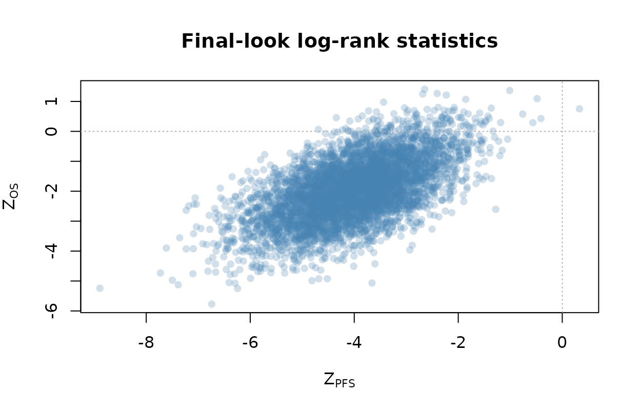
Standardized log-rank statistics at the final look.
Remarks
The cross-endpoint correlation at matching looks is moderate, around 0.6, and is largest at the first look, easing slightly as the trial matures. This cross-endpoint correlation is the input a sequential PFS-then-OS procedure needs to characterize its joint operating characteristics, and the simulation estimates it together with the power of the procedure. The within-endpoint correlations match the canonical group-sequential form to simulation error, which serves as a check on the event-driven timing and the shared-cutoff OS analysis.
The simulation uses the validated Rcpp primitives behind
analysis_fast for every log-rank computation, so the entire
study of 5,000 trials with three looks per endpoint runs in a few
seconds. Raising nsim tightens the correlation and power
estimates at a proportional cost.
References
Fleischer, F., Gaschler-Markefski, B., & Bluhmki, E. (2009). A statistical model for the dependence between progression-free survival and overall survival. Statistics in Medicine, 28(21), 2669-2686.
Glimm, E., Maurer, W., & Bretz, F. (2010). Hierarchical testing of multiple endpoints in group-sequential trials. Statistics in Medicine, 29(2), 219-228.
Lan, K. K. G., & DeMets, D. L. (1983). Discrete sequential boundaries for clinical trials. Biometrika, 70(3), 659-663.
O’Brien, P. C., & Fleming, T. R. (1979). A multiple testing procedure for clinical trials. Biometrics, 35(3), 549-556.
Pocock, S. J. (1977). Group sequential methods in the design and analysis of clinical trials. Biometrika, 64(2), 191-199.