Introduction to SingleArmMRCT

Background

Multi-regional clinical trials (MRCTs) are increasingly used in global drug development to allow simultaneous regulatory submissions across multiple regions. A key requirement for regional approval — particularly in Japan under the Japanese MHLW guidelines — is the demonstration of regional consistency: evidence that the treatment effect observed in a specific region (e.g., Japan) is consistent with the overall trial result.

Two widely used consistency evaluation methods, originally proposed under the Japanese guidelines, are:

Method 1 (Effect Retention Approach): Evaluates whether Region 1 retains at least a fraction $\pi$ of the overall treatment effect.
Method 2 (Simultaneous Positivity Approach): Evaluates whether all regional estimates simultaneously show a positive effect in the direction of benefit.

These methods were originally developed for two-arm randomised controlled trials. However, single-arm trials are now common in oncology and rare disease settings, where historical control comparisons are standard. The SingleArmMRCT package extends Method 1 and Method 2 to the single-arm setting, in which the treatment effect is defined relative to a pre-specified historical control value.

Regional Consistency Probability

The Regional Consistency Probability (RCP) is defined as the probability that a consistency criterion is satisfied, evaluated under the assumed true parameter values at the trial design stage. A trial design is said to have adequate regional consistency if the RCP exceeds a pre-specified target (commonly 0.80).

Method 1: Effect Retention Approach

Let $\theta$ denote the endpoint parameter for a given endpoint (e.g., mean, proportion, rate). Method 1 requires that Region 1 retains at least a fraction $\pi$ of the overall treatment effect:

$\text{RCP}_1 = \Pr\!\left[\,(\hat{\theta}_1 - \theta_0) \geq \pi \times (\hat{\theta} - \theta_0)\,\right]$

where $\hat{\theta}_1$ is the treatment effect estimate for Region 1, $\hat{\theta}$ is the overall pooled estimate, $\theta_0$ is the null (historical control) value, and $\pi \in [0, 1]$ is the pre-specified retention threshold (typically $\pi = 0.5$ ).

The consistency condition can be rewritten as $D \geq 0$ , where:

$D = \bigl(1 - \pi f_1\bigr)\,(\hat{\theta}_1 - \theta_0) - \pi(1 - f_1)\,(\hat{\theta}_{-1} - \theta_0)$

with $f_1 = N_1/N$ being the regional allocation fraction and $\hat{\theta}_{-1}$ the pooled estimate for regions $2, \ldots, J$ combined. Under the assumption of homogeneous treatment effects across regions, $D$ follows a normal distribution with mean $(1-\pi)\delta$ and a variance that depends on the endpoint type, yielding a closed-form expression for $\text{RCP}_1$ , where $\delta = \theta - \theta_0$ is the treatment effect.

For endpoints where a smaller value indicates benefit (e.g., hazard ratio, rate ratio), the inequality direction is reversed. See the endpoint-specific vignettes for exact formulae.

Method 2: Simultaneous Positivity Approach

Method 2 requires that all $J$ regional estimates simultaneously demonstrate a positive effect. For endpoints where a larger value indicates benefit (continuous, binary, milestone survival, RMST):

$\text{RCP}_2 = \Pr\!\left[\,\hat{\theta}_j > \theta_0 \;\text{ for all } j = 1, \ldots, J\,\right]$

For endpoints where a smaller value indicates benefit (hazard ratio, rate ratio):

$\text{RCP}_2 = \Pr\!\left[\,\hat{\theta}_j < \theta_0 \;\text{ for all } j = 1, \ldots, J\,\right]$

Because regional estimators are independent across regions, $\text{RCP}_2$ factorises as:

$\text{RCP}_2 = \prod_{j=1}^{J} \Pr\!\left[\,\hat{\theta}_j \text{ shows benefit}\,\right]$

Package Structure

The package provides a pair of functions for each of six endpoint types.

Endpoint	Calculation function	Plot function
Continuous	rcp1armContinuous()	plot_rcp1armContinuous()
Binary	rcp1armBinary()	plot_rcp1armBinary()
Count (negative binomial)	rcp1armCount()	plot_rcp1armCount()
Time-to-event (hazard ratio)	rcp1armHazardRatio()	plot_rcp1armHazardRatio()
Milestone survival	rcp1armMilestoneSurvival()	plot_rcp1armMilestoneSurvival()
Restricted mean survival time (RMST)	rcp1armRMST()	plot_rcp1armRMST()

Each calculation function supports two approaches:

"formula": Closed-form or semi-analytical solution based on normal approximation. Computationally fast and, for binary and count endpoints, exact.
"simulation": Monte Carlo simulation. Serves as an independent numerical check of the formula results.

Common Parameters

All six calculation functions share the following parameters.

Parameter	Type	Default	Description
`Nj`	integer vector	—	Sample sizes for each region; length equals the number of regions $J$
`PI`	numeric	`0.5`	Effect retention threshold $\pi$ for Method 1; must be in $[0, 1]$
`approach`	character	`"formula"`	Calculation approach: `"formula"` or `"simulation"`
`nsim`	integer	`10000`	Number of Monte Carlo iterations; used only when `approach = "simulation"`
`seed`	integer	`1`	Random seed for reproducibility; used only when `approach = "simulation"`

Time-to-event endpoints (hazard ratio, milestone survival, RMST) additionally require the following trial design parameters.

Parameter	Type	Default	Description
`t_a`	numeric	—	Accrual period: duration over which patients are uniformly enrolled
`t_f`	numeric	—	Follow-up period: additional observation time after accrual closes; total study duration is $\tau = t_a + t_f$
`lambda_dropout`	numeric or `NULL`	`NULL`	Exponential dropout hazard rate; `NULL` assumes no dropout

Quick Start Example

The following example computes RCP for a continuous endpoint with the setting below:

Parameter	Value
Total sample size	$N = 100$ ( $J = 2$ regions)
Region 1 allocation	$N_1 = 10$ ( $f_1 = 10\%$ )
True mean	$\mu = 0.5$
Historical control mean	$\mu_0 = 0.1$ (mean difference $\delta = 0.4$ )
Standard deviation	$\sigma = 1$
Retention threshold	$\pi = 0.5$

Closed-form solution

result_formula <- rcp1armContinuous(
  mu       = 0.5,
  mu0      = 0.1,
  sd       = 1,
  Nj       = c(10, 90),
  PI       = 0.5,
  approach = "formula"
)
print(result_formula)
#> 
#> Regional Consistency Probability for Single-Arm MRCT
#> Endpoint : Continuous
#> 
#>    Approach    : Closed-Form Solution
#>    Target Mean : mu  = 0.5000
#>    Null Mean   : mu0 = 0.1000
#>    Std. Dev.   : sd  = 1.0000
#>    Sample Size : Nj  = (10, 90)
#>    Total Size  : N   = 100
#>    Threshold   : PI  = 0.5000
#> 
#> Consistency Probabilities:
#>    Method 1 (Region 1 vs Overall)  : 0.7446
#>    Method 2 (All Regions > mu0)    : 0.8970

Monte Carlo simulation

result_sim <- rcp1armContinuous(
  mu       = 0.5,
  mu0      = 0.1,
  sd       = 1,
  Nj       = c(10, 90),
  PI       = 0.5,
  approach = "simulation",
  nsim     = 10000,
  seed     = 1
)
print(result_sim)
#> 
#> Regional Consistency Probability for Single-Arm MRCT
#> Endpoint : Continuous
#> 
#>    Approach    : Simulation-Based (nsim = 10000)
#>    Target Mean : mu  = 0.5000
#>    Null Mean   : mu0 = 0.1000
#>    Std. Dev.   : sd  = 1.0000
#>    Sample Size : Nj  = (10, 90)
#>    Total Size  : N   = 100
#>    Threshold   : PI  = 0.5000
#> 
#> Consistency Probabilities:
#>    Method 1 (Region 1 vs Overall)  : 0.7421
#>    Method 2 (All Regions > mu0)    : 0.8922

The closed-form and simulation results are in close agreement. The small difference is attributable to Monte Carlo sampling variation and diminishes as nsim increases.

Visualisation

Each endpoint type has a corresponding plot_rcp1arm*() function. These functions display RCP as a function of the regional allocation proportion $f_1 = N_1/N$ , with separate facets for different total sample sizes $N$ . Both Method 1 (blue) and Method 2 (yellow) are shown, with solid lines for the formula approach and dashed lines for simulation. The horizontal grey dashed line marks the commonly used design target of RCP $= 0.80$ .

The base_size argument controls font size: use the default (base_size = 28) for presentation slides, and a smaller value (e.g., base_size = 11) for documents and vignettes.

plot_rcp1armContinuous(
  mu        = 0.5,
  mu0       = 0.1,
  sd        = 1,
  PI        = 0.5,
  N_vec     = c(20, 40, 100),
  J         = 3,
  nsim      = 5000,
  seed      = 1,
  base_size = 11
)

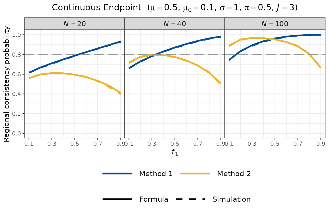
Line plot of RCP versus regional allocation proportion f1 for a continuous endpoint, comparing Method 1 and Method 2 using formula and simulation approaches across sample sizes N = 20, 40, and 100

Several features are evident from the plot:

Method 1 (blue) increases with $f_1$ : as Region 1 becomes larger, its estimator $\hat{\theta}_1$ becomes more precise, making the retention condition easier to satisfy.
Method 2 (yellow) is maximised when all regions have equal allocation $f_1 = f_2 = \cdots = f_J = 1/J$ , and decreases as $f_1$ deviates from this balance, because unequal allocation reduces the marginal probability $\Pr(\hat{\theta}_j \text{ shows benefit})$ for the smaller regions.
Both RCP values increase with total sample size $N$ , as expected.
The formula (solid) and simulation (dashed) curves are closely aligned, confirming the accuracy of the normal approximation.

References

Hayashi N, Itoh Y (2017). A re-examination of Japanese sample size calculation for multi-regional clinical trial evaluating survival endpoint. Japanese Journal of Biometrics, 38(2): 79–92. https://doi.org/10.5691/jjb.38.79

Homma G (2024). Cautionary note on regional consistency evaluation in multiregional clinical trials with binary outcomes. Pharmaceutical Statistics, 23(3):385–398. https://doi.org/10.1002/pst.2358

Wu J (2015). Sample size calculation for the one-sample log-rank test. Pharmaceutical Statistics, 14(1): 26–33. https://doi.org/10.1002/pst.1654