Survival Endpoints: Hazard Ratio, Milestone Survival, and RMST

This vignette describes Regional Consistency Probability (RCP) calculations for three survival endpoint types: hazard ratio, milestone survival probability, and restricted mean survival time (RMST). All three endpoints share a common trial design framework, and event times are modelled by the exponential distribution.

---

Common trial design framework

For all survival endpoints, the following parameters define the trial design.

Parameter	Symbol	Description
t_a	$t_a$	Accrual period; patients enrol uniformly over $[0, t_a]$
t_f	$t_f$	Follow-up period after accrual closes
tau	$\tau = t_a + t_f$	Total study duration (computed internally)
lambda	$\lambda$	True hazard rate under the alternative (exponential model)
lambda0	$\lambda_0$	Historical control hazard rate
lambda_dropout	$\lambda_d$	Dropout hazard rate; NULL assumes no dropout (default)

The common parameters below are used throughout the examples in this vignette.

lambda  <- log(2) / 10   # treatment arm: median survival = 10
lambda0 <- log(2) / 5    # historical control: median survival = 5
t_a     <- 3             # accrual period
t_f     <- 10            # follow-up period
# True HR = lambda / lambda0 = 0.5

---

1. Hazard Ratio Endpoint

Statistical model

Under the exponential model with uniform accrual over $[0, t_a]$ and administrative censoring at $\tau$, the expected event probability per patient is:

$$\phi = \frac{\lambda}{\lambda + \lambda_d} \left[1 - \frac{e^{-(\lambda + \lambda_d)t_f} - e^{-(\lambda + \lambda_d)\tau}}{(\lambda + \lambda_d)\,t_a}\right]$$

The expected number of events in Region $j$ is $E_j = N_j\,\phi$, and the log-hazard ratio estimator has the approximate distribution:

$$\log(\widehat{HR}_j) \sim N\!\left(\log(HR),\; \frac{1}{E_j}\right)$$

Consistency criteria

Method 1 (log-HR scale):

Letting $\delta = \log(HR) < 0$, $E_1 = N_1\phi$, and $E_{-1} = (N - N_1)\phi$:

$$\text{RCP}_{1,\log} = \Phi\!\left(\frac{-(1 - \pi)\,\delta} {\sqrt{(1 - \pi f_1)^2/E_1 + \{\pi(1 - f_1)\}^2/E_{-1}}}\right)$$

Method 1 (linear-HR scale) (Hayashi and Itoh 2018):

$$\text{RCP}_{1,\text{lin}} = \Pr\!\left[\,(1 - \widehat{HR}_1) \geq \pi\,(1 - \widehat{HR})\,\right]$$

This is derived via the delta method. Define $g = \log(\widehat{HR}_1) - \log(1 - \pi + \pi\,\widehat{HR})$. Under homogeneity:

$$E[g] = \log(HR) - \log(1 - \pi + \pi\,HR)$$

$$\mathrm{Var}(g) = \frac{1}{E_{\text{total}}} \left[ \frac{\{1 - \pi + \pi(1 - f_1)HR\}^2}{f_1\,(1 - \pi + \pi\,HR)^2} + \frac{\{\pi(1 - f_1)HR\}^2}{(1 - f_1)\,(1 - \pi + \pi\,HR)^2} \right]$$

and $\text{RCP}_{1,\text{lin}} = \Phi(-E[g] / \sqrt{\mathrm{Var}(g)})$.

Method 2:

$$\text{RCP}_2 = \prod_{j=1}^{J} \Pr\!\left(\widehat{HR}_j < 1\right) = \prod_{j=1}^{J} \Phi\!\left(-\delta\,\sqrt{E_j}\right)$$

Example

result_f <- rcp1armHazardRatio(
  lambda         = lambda,
  lambda0        = lambda0,
  Nj             = c(20, 80),
  t_a            = t_a,
  t_f            = t_f,
  lambda_dropout = NULL,
  PI             = 0.5,
  approach       = "formula"
)
print(result_f)
#> 
#> Regional Consistency Probability for Single-Arm MRCT
#> Endpoint : Time-to-Event (Hazard Ratio)
#> 
#>    Approach       : Closed-Form Solution
#>    True Hazard    : lambda  = 0.069315
#>    Control Hazard : lambda0 = 0.138629
#>    Sample Size    : Nj      = (20, 80)
#>    Total Size     : N       = 100
#>    Accrual Period : t_a     = 3.00
#>    Follow-up      : t_f     = 10.00
#>    Study Duration : tau     = 13.00
#>    Dropout Hazard : lambda_d = NA
#>    Threshold      : PI      = 0.5000
#> 
#> Consistency Probabilities:
#>    Method 1 (Region 1 vs Overall):
#>       Log-HR based    : 0.8935
#>       Linear-HR based : 0.9228
#>    Method 2 (All Regions Show Benefit):
#>       HR < 1          : 0.9892

result_s <- rcp1armHazardRatio(
  lambda         = lambda,
  lambda0        = lambda0,
  Nj             = c(20, 80),
  t_a            = t_a,
  t_f            = t_f,
  lambda_dropout = NULL,
  PI             = 0.5,
  approach       = "simulation",
  nsim           = 10000,
  seed           = 1
)
print(result_s)
#> 
#> Regional Consistency Probability for Single-Arm MRCT
#> Endpoint : Time-to-Event (Hazard Ratio)
#> 
#>    Approach       : Simulation-Based (nsim = 10000)
#>    True Hazard    : lambda  = 0.069315
#>    Control Hazard : lambda0 = 0.138629
#>    Sample Size    : Nj      = (20, 80)
#>    Total Size     : N       = 100
#>    Accrual Period : t_a     = 3.00
#>    Follow-up      : t_f     = 10.00
#>    Study Duration : tau     = 13.00
#>    Dropout Hazard : lambda_d = NA
#>    Threshold      : PI      = 0.5000
#> 
#> Consistency Probabilities:
#>    Method 1 (Region 1 vs Overall):
#>       Log-HR based    : 0.9019
#>       Linear-HR based : 0.9320
#>    Method 2 (All Regions Show Benefit):
#>       HR < 1          : 0.9924

Effect of dropout

Specifying lambda_dropout reduces the expected event probability $\phi$, which in turn reduces all RCP values.

result_dropout <- rcp1armHazardRatio(
  lambda         = lambda,
  lambda0        = lambda0,
  Nj             = c(20, 80),
  t_a            = t_a,
  t_f            = t_f,
  lambda_dropout = 0.05,
  PI             = 0.5,
  approach       = "formula"
)
print(result_dropout)
#> 
#> Regional Consistency Probability for Single-Arm MRCT
#> Endpoint : Time-to-Event (Hazard Ratio)
#> 
#>    Approach       : Closed-Form Solution
#>    True Hazard    : lambda  = 0.069315
#>    Control Hazard : lambda0 = 0.138629
#>    Sample Size    : Nj      = (20, 80)
#>    Total Size     : N       = 100
#>    Accrual Period : t_a     = 3.00
#>    Follow-up      : t_f     = 10.00
#>    Study Duration : tau     = 13.00
#>    Dropout Hazard : lambda_d = 0.050000
#>    Threshold      : PI      = 0.5000
#> 
#> Consistency Probabilities:
#>    Method 1 (Region 1 vs Overall):
#>       Log-HR based    : 0.8656
#>       Linear-HR based : 0.8971
#>    Method 2 (All Regions Show Benefit):
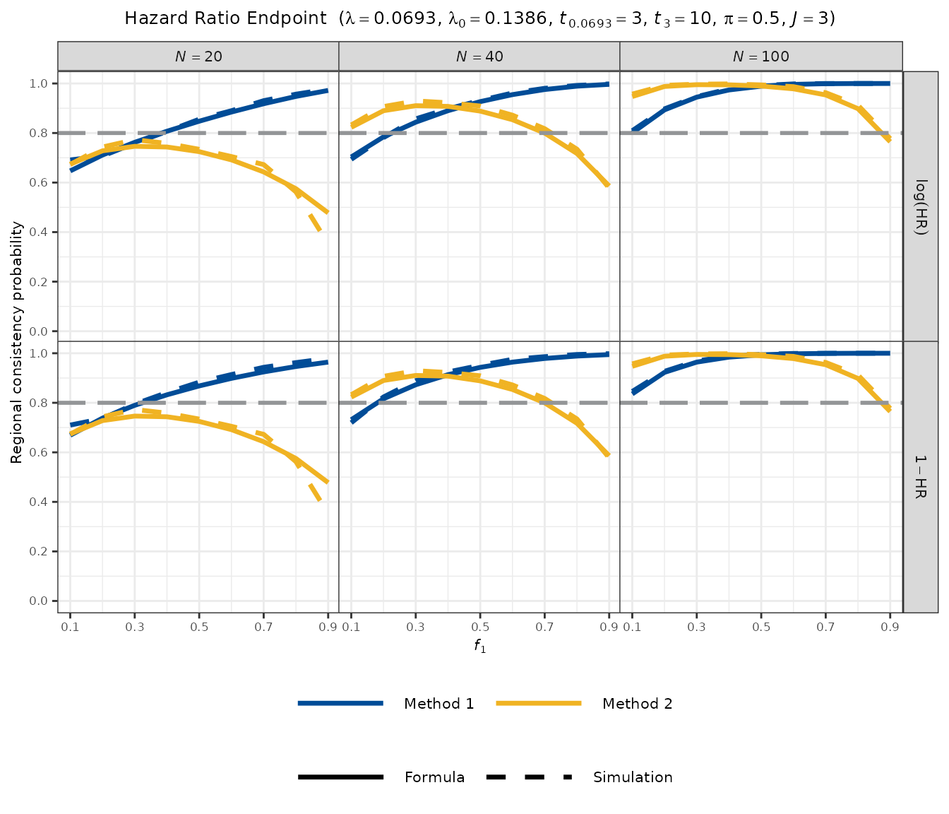
#>       HR < 1          : 0.9793

Visualisation

plot_rcp1armHazardRatio(
  lambda    = lambda,
  lambda0   = lambda0,
  t_a       = t_a,
  t_f       = t_f,
  PI        = 0.5,
  N_vec     = c(20, 40, 100),
  J         = 3,
  nsim      = 5000,
  seed      = 1,
  base_size = 8
)

---

2. Milestone Survival Endpoint

Statistical model

The treatment effect at evaluation time $t_{\text{eval}}$ is:

$$\delta = S(t_{\text{eval}}) - S_0 = e^{-\lambda\,t_{\text{eval}}} - S_0$$

where $S_0$ is the historical control survival rate at $t_{\text{eval}}$, supplied by the user.

The asymptotic variance of the Kaplan-Meier estimator $\hat{S}_j(t_{\text{eval}})$ is derived from Greenwood’s formula:

$$\mathrm{Var}\!\left[\hat{S}_j(t)\right] \approx \frac{e^{-2\lambda t}}{N_j} \int_0^{t} \frac{\lambda\,e^{(\lambda + \lambda_d)u}}{G_a(u)}\,du \;=:\; \frac{v_{KM}(t)}{N_j}$$

where:

$$G_a(u) = \begin{cases} 1 & 0 \leq u \leq t_f \\ (\tau - u)/t_a & t_f < u \leq \tau \end{cases}$$

Closed-form solution when $t_{\text{eval}} \leq t_f$ ($G_a(u) = 1$ throughout):

$$v_{KM}(t) = e^{-2\lambda t} \cdot \frac{\lambda}{\lambda + \lambda_d} \left(e^{(\lambda + \lambda_d)\,t} - 1\right)$$

For $\lambda_d = 0$ this reduces to the binomial variance $S(t)(1 - S(t))$. When $t_{\text{eval}} > t_f$, the integral is evaluated numerically via stats::integrate().

Consistency criteria

Method 1:

$$\text{RCP}_1 = \Phi\!\left(\frac{(1 - \pi)\,\delta} {\sqrt{(1 - \pi f_1)^2\,v_{KM}/N_1 + \{\pi(1 - f_1)\}^2\,v_{KM}/(N - N_1)}}\right)$$

Method 2:

$$\text{RCP}_2 = \prod_{j=1}^{J} \Phi\!\left(\frac{\delta}{\sqrt{v_{KM}/N_j}}\right)$$

Example

t_eval <- 8
S0     <- exp(-log(2) * t_eval / 5)
cat(sprintf("True S(%g) = %.4f,  S0 = %.4f,  delta = %.4f\n",
            t_eval, exp(-lambda * t_eval), S0,
            exp(-lambda * t_eval) - S0))
#> True S(8) = 0.5743,  S0 = 0.3299,  delta = 0.2445

result_f <- rcp1armMilestoneSurvival(
  lambda         = lambda,
  t_eval         = t_eval,
  S0             = S0,
  Nj             = c(20, 80),
  t_a            = t_a,
  t_f            = t_f,
  lambda_dropout = NULL,
  PI             = 0.5,
  approach       = "formula"
)
print(result_f)
#> 
#> Regional Consistency Probability for Single-Arm MRCT
#> Endpoint : Milestone Survival
#> 
#>    Approach       : Closed-Form Solution (Greenwood)
#>    True Hazard    : lambda  = 0.069315
#>    Sample Size    : Nj      = (20, 80)
#>    Total Size     : N       = 100
#>    Accrual Period : t_a     = 3.00
#>    Follow-up      : t_f     = 10.00
#>    Study Duration : tau     = 13.00
#>    Dropout Hazard : lambda_d = NA
#>    Threshold      : PI      = 0.5000
#>    Eval Time      : t_eval  = 8.00
#>    Control Surv   : S0      = 0.3299
#>    True Surv      : S_est   = 0.5743
#> 
#> Consistency Probabilities:
#>    Method 1 (Region 1 vs Overall)  : 0.8848
#>    Method 2 (All Regions > S0)     : 0.9865

Since $t_{\text{eval}} = 8 \leq t_f = 10$, the closed-form solution is used (formula_type = "closed-form"). For $t_{\text{eval}} > t_f$, numerical integration is applied automatically.

result_s <- rcp1armMilestoneSurvival(
  lambda         = lambda,
  t_eval         = t_eval,
  S0             = S0,
  Nj             = c(20, 80),
  t_a            = t_a,
  t_f            = t_f,
  lambda_dropout = NULL,
  PI             = 0.5,
  approach       = "simulation",
  nsim           = 10000,
  seed           = 1
)
print(result_s)
#> 
#> Regional Consistency Probability for Single-Arm MRCT
#> Endpoint : Milestone Survival
#> 
#>    Approach       : Simulation-Based (nsim = 10000)
#>    True Hazard    : lambda  = 0.069315
#>    Sample Size    : Nj      = (20, 80)
#>    Total Size     : N       = 100
#>    Accrual Period : t_a     = 3.00
#>    Follow-up      : t_f     = 10.00
#>    Study Duration : tau     = 13.00
#>    Dropout Hazard : lambda_d = NA
#>    Threshold      : PI      = 0.5000
#>    Eval Time      : t_eval  = 8.00
#>    Control Surv   : S0      = 0.3299
#>    True Surv      : S_est   = 0.5743
#> 
#> Consistency Probabilities:
#>    Method 1 (Region 1 vs Overall)  : 0.8873
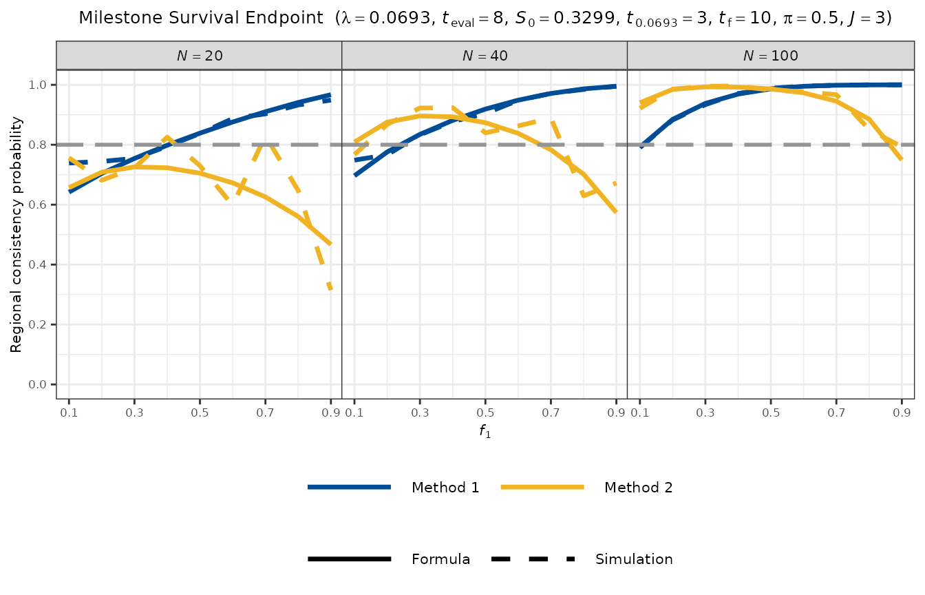
#>    Method 2 (All Regions > S0)     : 0.9887

Visualisation

plot_rcp1armMilestoneSurvival(
  lambda    = lambda,
  t_eval    = t_eval,
  S0        = S0,
  t_a       = t_a,
  t_f       = t_f,
  PI        = 0.5,
  N_vec     = c(20, 40, 100),
  J         = 3,
  nsim      = 5000,
  seed      = 1,
  base_size = 8
)

---

3. RMST Endpoint

Statistical model

The restricted mean survival time (RMST) up to truncation time $\tau^*$ is:

$$\mu(\tau^*) = \int_0^{\tau^*} S(t)\,dt = \frac{1 - e^{-\lambda\tau^*}}{\lambda}$$

The asymptotic variance of the regional RMST estimator is:

$$\mathrm{Var}\!\left[\hat{\mu}_j(\tau^*)\right] \approx \frac{v_{\text{RMST}}(\tau^*)}{N_j}$$

where:

$$v_{\text{RMST}}(\tau^*) = \int_0^{\tau^*} \frac{e^{\lambda_d t}\left(1 - e^{-\lambda(\tau^* - t)}\right)^2}{\lambda\,G_a(t)}\,dt$$

Closed-form solution when $\tau^* \leq t_f$, using $A(r) = (e^{r\tau^*} - 1)/r$ (and $A(0) = \tau^*$):

$$ v_{\text{RMST}}(\tau^*) = \frac{1}{\lambda}\Bigl[ A(\lambda_d) - 2\,e^{-\lambda\tau^*}\,A(\lambda_d + \lambda) + e^{-2\lambda\tau^*}\,A(\lambda_d + 2\lambda) \Bigr] $$

For $\lambda_d = 0$ this simplifies to:

$$v_{\text{RMST}}(\tau^*) = \tau^* - \frac{2(1 - e^{-\lambda\tau^*})}{\lambda} + \frac{1 - e^{-2\lambda\tau^*}}{2\lambda}$$

When $\tau^* > t_f$, the integral is split at $t_f$ and evaluated via stats::integrate().

Consistency criteria

Method 1:

$$\text{RCP}_1 = \Phi\!\left(\frac{(1 - \pi)\,(\mu_{\text{est}} - \mu_0)} {\sqrt{(1 - \pi f_1)^2\,v/N_1 + \{\pi(1 - f_1)\}^2\,v/(N - N_1)}}\right)$$

Method 2:

$$\text{RCP}_2 = \prod_{j=1}^{J} \Phi\!\left(\frac{\mu_{\text{est}} - \mu_0}{\sqrt{v/N_j}}\right)$$

Example

tau_star <- 8
mu0      <- (1 - exp(-lambda0 * tau_star)) / lambda0
mu_est   <- (1 - exp(-lambda  * tau_star)) / lambda
cat(sprintf("True RMST = %.4f,  mu0 = %.4f,  delta = %.4f\n",
            mu_est, mu0, mu_est - mu0))
#> True RMST = 6.1408,  mu0 = 4.8339,  delta = 1.3069

result_f <- rcp1armRMST(
  lambda         = lambda,
  tau_star       = tau_star,
  mu0            = mu0,
  Nj             = c(20, 80),
  t_a            = t_a,
  t_f            = t_f,
  lambda_dropout = NULL,
  PI             = 0.5,
  approach       = "formula"
)
print(result_f)
#> 
#> Regional Consistency Probability for Single-Arm MRCT
#> Endpoint : Restricted Mean Survival Time (RMST)
#> 
#>    Approach       : Closed-Form Solution
#>    True Hazard    : lambda  = 0.069315
#>    Sample Size    : Nj      = (20, 80)
#>    Total Size     : N       = 100
#>    Accrual Period : t_a     = 3.00
#>    Follow-up      : t_f     = 10.00
#>    Study Duration : tau     = 13.00
#>    Dropout Hazard : lambda_d = NA
#>    Threshold      : PI      = 0.5000
#>    Trunc. Time    : tau*    = 8.00
#>    Control RMST   : mu0     = 4.8339
#>    True RMST      : mu_est  = 6.1408
#> 
#> Consistency Probabilities:
#>    Method 1 (Region 1 vs Overall)  : 0.8693
#>    Method 2 (All Regions > mu0)    : 0.9808

result_s <- rcp1armRMST(
  lambda         = lambda,
  tau_star       = tau_star,
  mu0            = mu0,
  Nj             = c(20, 80),
  t_a            = t_a,
  t_f            = t_f,
  lambda_dropout = NULL,
  PI             = 0.5,
  approach       = "simulation",
  nsim           = 10000,
  seed           = 1
)
print(result_s)
#> 
#> Regional Consistency Probability for Single-Arm MRCT
#> Endpoint : Restricted Mean Survival Time (RMST)
#> 
#>    Approach       : Simulation-Based (nsim = 10000)
#>    True Hazard    : lambda  = 0.069315
#>    Sample Size    : Nj      = (20, 80)
#>    Total Size     : N       = 100
#>    Accrual Period : t_a     = 3.00
#>    Follow-up      : t_f     = 10.00
#>    Study Duration : tau     = 13.00
#>    Dropout Hazard : lambda_d = NA
#>    Threshold      : PI      = 0.5000
#>    Trunc. Time    : tau*    = 8.00
#>    Control RMST   : mu0     = 4.8339
#>    True RMST      : mu_est  = 6.1408
#> 
#> Consistency Probabilities:
#>    Method 1 (Region 1 vs Overall)  : 0.8790
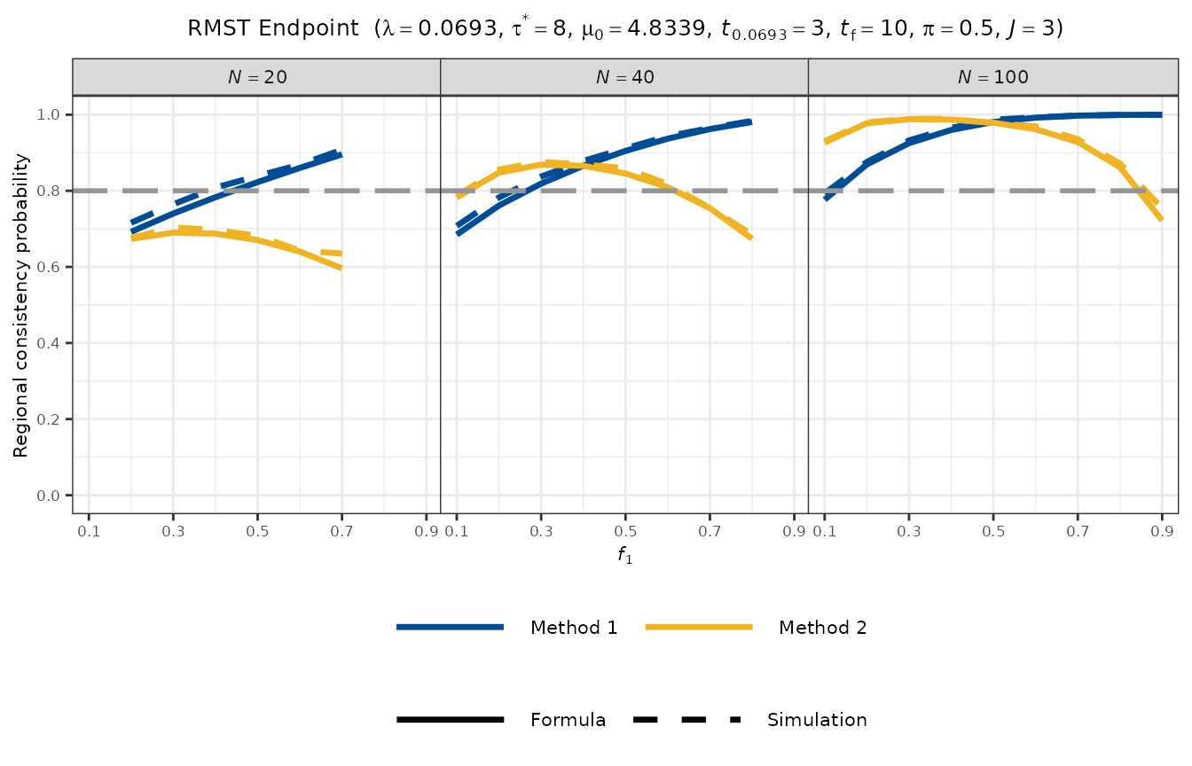
#>    Method 2 (All Regions > mu0)    : 0.9809

Visualisation

plot_rcp1armRMST(
  lambda    = lambda,
  tau_star  = tau_star,
  mu0       = mu0,
  t_a       = t_a,
  t_f       = t_f,
  PI        = 0.5,
  N_vec     = c(20, 40, 100),
  J         = 3,
  nsim      = 5000,
  seed      = 1,
  base_size = 8
)

---

Summary

Endpoint	Effect parameter	Benefit direction	Variance basis	Closed-form condition
Hazard Ratio	$\log(HR) = \log(\lambda/\lambda_0)$ (Method 1, log-HR scale); $1 - HR = 1 - \lambda/\lambda_0$ (Method 1, linear-HR scale)	$\widehat{HR}_j < 1$	Expected events via $\phi$ (Wu 2015)	Always
Milestone Survival	$\delta = e^{-\lambda t_{\text{eval}}} - S_0$	$\hat{S}_j(t) > S_0$	Greenwood’s formula	$t_{\text{eval}} \leq t_f$
RMST	$\delta = \mu(\tau^*) - \mu_0(\tau^*)$	$\hat{\mu}_j > \mu_0$	Squared survival difference integral	$\tau^* \leq t_f$

---

References

Hayashi N, Itoh Y (2017). A re-examination of Japanese sample size calculation for multi-regional clinical trial evaluating survival endpoint. Japanese Journal of Biometrics, 38(2): 79–92. https://doi.org/10.5691/jjb.38.79

Wu J (2015). Sample size calculation for the one-sample log-rank test. Pharmaceutical Statistics, 14(1): 26–33. https://doi.org/10.1002/pst.1654