Non-Survival Endpoints: Continuous, Binary, and Count

This vignette describes Regional Consistency Probability (RCP) calculations for three non-survival endpoint types: continuous, binary, and count (negative binomial). For each endpoint, the statistical model, treatment effect scale, closed-form formulae, and worked examples are provided.

---

1. Continuous Endpoint

Statistical model

Let $\hat{\mu}_j$ denote the sample mean for Region $j$. Under the assumption that individual observations are independently and identically distributed as $N(\mu, \sigma^2)$ within each region, the regional sample means are:

$$\hat{\mu}_j \sim N\!\left(\mu,\; \frac{\sigma^2}{N_j}\right), \qquad j = 1, \ldots, J$$

independently across regions. The treatment effect relative to a historical control mean $\mu_0$ is $\delta = \mu - \mu_0 > 0$.

Consistency criteria

Method 1 (Effect Retention):

$$\text{RCP}_1 = \Pr\!\left[\,(\hat{\mu}_1 - \mu_0) \geq \pi\,(\hat{\mu} - \mu_0)\,\right]$$

Defining $D = (\hat{\mu}_1 - \mu_0) - \pi(\hat{\mu} - \mu_0)$, the condition $D \geq 0$ is equivalent to:

$$D = (1 - \pi f_1)\,(\hat{\mu}_1 - \mu_0) - \pi(1 - f_1)\,(\hat{\mu}_{-1} - \mu_0) \geq 0$$

where $\hat{\mu}_{-1}$ is the sample mean pooled over regions $2, \ldots, J$. Under homogeneity:

$$E[D] = (1 - \pi)\,\delta, \qquad \mathrm{Var}(D) = (1 - \pi f_1)^2\,\frac{\sigma^2}{N_1} + \bigl[\pi(1 - f_1)\bigr]^2\,\frac{\sigma^2}{N - N_1}$$

Therefore:

$$\text{RCP}_1 = \Phi\!\left(\frac{(1 - \pi)\,\delta} {\sqrt{(1 - \pi f_1)^2\,\sigma^2/N_1 + \{\pi(1 - f_1)\}^2\,\sigma^2/(N - N_1)}}\right)$$

Method 2 (Simultaneous Positivity):

$$\text{RCP}_2 = \Pr\!\left[\,\hat{\mu}_j > \mu_0 \;\text{ for all } j\,\right] = \prod_{j=1}^{J} \Phi\!\left(\frac{\delta\,\sqrt{N_j}}{\sigma}\right)$$

Example

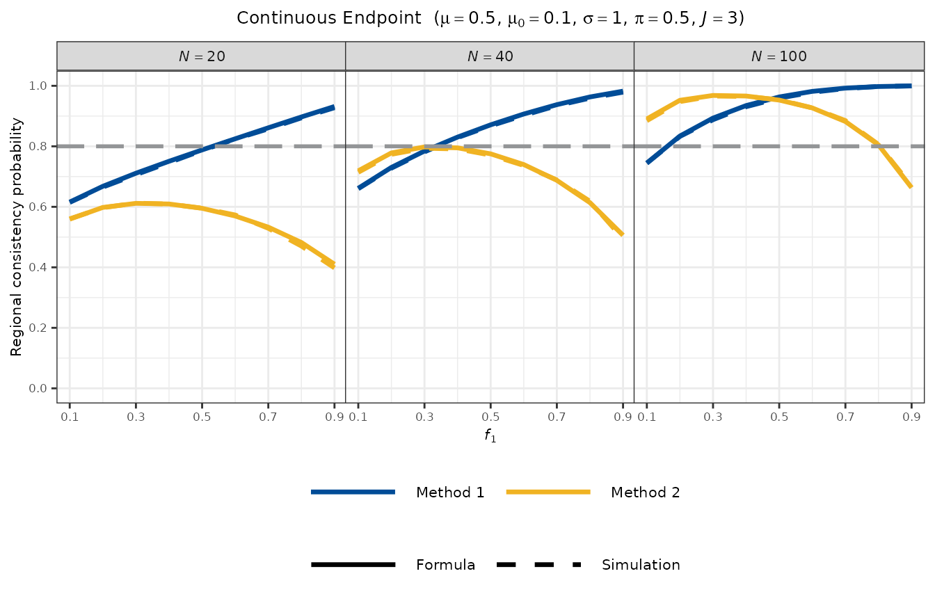
Setting: $\mu = 0.5$, $\mu_0 = 0.1$, $\sigma = 1$, $N = 100$ ($J = 3$ regions with $N_1 = 20$), $\pi = 0.5$.

result_f <- rcp1armContinuous(
  mu       = 0.5,
  mu0      = 0.1,
  sd       = 1,
  Nj       = c(20, 40, 40),
  PI       = 0.5,
  approach = "formula"
)
print(result_f)
#> 
#> Regional Consistency Probability for Single-Arm MRCT
#> Endpoint : Continuous
#> 
#>    Approach    : Closed-Form Solution
#>    Target Mean : mu  = 0.5000
#>    Null Mean   : mu0 = 0.1000
#>    Std. Dev.   : sd  = 1.0000
#>    Sample Size : Nj  = (20, 40, 40)
#>    Total Size  : N   = 100
#>    Threshold   : PI  = 0.5000
#> 
#> Consistency Probabilities:
#>    Method 1 (Region 1 vs Overall)  : 0.8340
#>    Method 2 (All Regions > mu0)    : 0.9522

result_s <- rcp1armContinuous(
  mu       = 0.5,
  mu0      = 0.1,
  sd       = 1,
  Nj       = c(20, 40, 40),
  PI       = 0.5,
  approach = "simulation",
  nsim     = 10000,
  seed     = 1
)
print(result_s)
#> 
#> Regional Consistency Probability for Single-Arm MRCT
#> Endpoint : Continuous
#> 
#>    Approach    : Simulation-Based (nsim = 10000)
#>    Target Mean : mu  = 0.5000
#>    Null Mean   : mu0 = 0.1000
#>    Std. Dev.   : sd  = 1.0000
#>    Sample Size : Nj  = (20, 40, 40)
#>    Total Size  : N   = 100
#>    Threshold   : PI  = 0.5000
#> 
#> Consistency Probabilities:
#>    Method 1 (Region 1 vs Overall)  : 0.8338
#>    Method 2 (All Regions > mu0)    : 0.9479

Visualisation

plot_rcp1armContinuous(
  mu        = 0.5,
  mu0       = 0.1,
  sd        = 1,
  PI        = 0.5,
  N_vec     = c(20, 40, 100),
  J         = 3,
  nsim      = 5000,
  seed      = 1,
  base_size = 8
)

---

2. Binary Endpoint

Statistical model

Let $Y_j$ denote the number of responders in Region $j$. Under independent Bernoulli trials with a common response rate $p$:

$$Y_j \sim \mathrm{Binomial}(N_j,\; p), \qquad j = 1, \ldots, J$$

independently across regions. The regional response rate estimator is $\hat{p}_j = Y_j / N_j$, the overall estimator is $\hat{p} = \sum_j Y_j / N$, and the treatment effect is $\delta = p - p_0 > 0$.

Consistency criteria

Method 1 (Effect Retention) — Exact Enumeration:

$$\text{RCP}_1 = \Pr\!\left[\,(\hat{p}_1 - p_0) \geq \pi\,(\hat{p} - p_0)\,\right]$$

By the additivity of independent binomials, $Y_{-1} = \sum_{j \geq 2} Y_j \sim \mathrm{Binomial}(N - N_1,\; p)$. The formula approach enumerates all combinations $(y_1, y_{-1}) \in \{0, \ldots, N_1\} \times \{0, \ldots, N - N_1\}$ and sums the joint probabilities satisfying the consistency condition:

$$\text{RCP}_1 = \sum_{y_1=0}^{N_1} \sum_{y_{-1}=0}^{N-N_1} b(y_1;\,N_1,\,p)\;b(y_{-1};\,N{-}N_1,\,p) \cdot \mathbf{1}\!\left[\frac{y_1}{N_1} - p_0 \geq \pi\!\left(\frac{y_1+y_{-1}}{N} - p_0\right)\right]$$

where $b(y;\,n,\,p) = \binom{n}{y}p^y(1-p)^{n-y}$.

Method 2 (Simultaneous Positivity):

The condition $\hat{p}_j > p_0$ is equivalent to $Y_j \geq y_{j,\min}$ where $y_{j,\min} = \lfloor N_j p_0 \rfloor + 1$. Denoting by $F_{\mathrm{Bin}(n,\,p)}(k)$ the CDF of the binomial distribution with parameters $n$ and $p$ evaluated at $k$:

$$\text{RCP}_2 = \prod_{j=1}^{J} \left[1 - F_{\mathrm{Bin}(N_j,\,p)}(y_{j,\min} - 1)\right]$$

Example

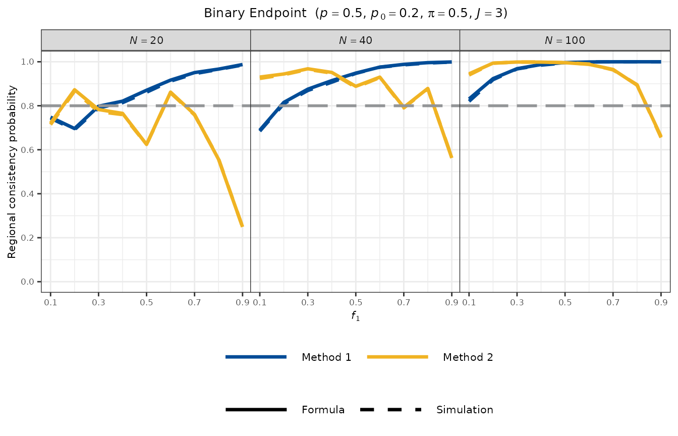
Setting: $p = 0.5$, $p_0 = 0.2$, $N = 100$ ($J = 3$ regions with $N_1 = 20$), $\pi = 0.5$.

result_f <- rcp1armBinary(
  p        = 0.5,
  p0       = 0.2,
  Nj       = c(20, 40, 40),
  PI       = 0.5,
  approach = "formula"
)
print(result_f)
#> 
#> Regional Consistency Probability for Single-Arm MRCT
#> Endpoint : Binary
#> 
#>    Approach      : Exact Solution
#>    Response Rate : p  = 0.5000
#>    Null Rate     : p0 = 0.2000
#>    Sample Size   : Nj = (20, 40, 40)
#>    Total Size    : N  = 100
#>    Threshold     : PI = 0.5000
#> 
#> Consistency Probabilities:
#>    Method 1 (Region 1 vs Overall) : 0.9234
#>    Method 2 (All Regions > p0)    : 0.9939

result_s <- rcp1armBinary(
  p        = 0.5,
  p0       = 0.2,
  Nj       = c(20, 40, 40),
  PI       = 0.5,
  approach = "simulation",
  nsim     = 10000,
  seed     = 1
)
print(result_s)
#> 
#> Regional Consistency Probability for Single-Arm MRCT
#> Endpoint : Binary
#> 
#>    Approach      : Simulation-Based (nsim = 10000)
#>    Response Rate : p  = 0.5000
#>    Null Rate     : p0 = 0.2000
#>    Sample Size   : Nj = (20, 40, 40)
#>    Total Size    : N  = 100
#>    Threshold     : PI = 0.5000
#> 
#> Consistency Probabilities:
#>    Method 1 (Region 1 vs Overall) : 0.9203
#>    Method 2 (All Regions > p0)    : 0.9933

Visualisation

plot_rcp1armBinary(
  p         = 0.5,
  p0        = 0.2,
  PI        = 0.5,
  N_vec     = c(20, 40, 100),
  J         = 3,
  nsim      = 5000,
  seed      = 1,
  base_size = 8
)

---

3. Count Endpoint (Negative Binomial)

Statistical model

Count data are modelled by the negative binomial distribution. The total event count in Region $j$ is:

$$Y_j \sim \mathrm{NB}\!\left(\mu = N_j\,\lambda,\;\; \mathrm{size} = N_j\,\phi\right), \qquad j = 1, \ldots, J$$

independently across regions, where $\lambda > 0$ is the expected count per patient under the alternative and $\phi > 0$ is the dispersion parameter. The regional rate estimator is $\hat{\lambda}_j = Y_j / N_j$, and the treatment effect is expressed as a rate ratio:

$$\widehat{RR}_j = \frac{\hat{\lambda}_j}{\lambda_0}$$

Benefit is indicated by $RR = \lambda / \lambda_0 < 1$.

By the reproducibility property of the negative binomial, the pooled count for regions $2, \ldots, J$ follows $\mathrm{NB}(\mu = (N - N_1)\lambda,\; \mathrm{size} = (N - N_1)\phi)$, enabling exact enumeration analogous to the binary case.

Consistency criteria

Method 1 (log-RR scale):

$$\text{RCP}_{1,\log} = \Pr\!\left[\,\log(\widehat{RR}_1) \leq \pi\,\log(\widehat{RR})\,\right]$$

Since $RR < 1$ (benefit), $\log(RR) < 0$, so the condition requires $\log(\widehat{RR}_1)$ to be sufficiently negative relative to the overall $\log(\widehat{RR})$.

Method 1 (linear-RR scale):

$$\text{RCP}_{1,\text{lin}} = \Pr\!\left[\,(1 - \widehat{RR}_1) \geq \pi\,(1 - \widehat{RR})\,\right]$$

Both Method 1 variants use exact enumeration over all $(y_1, y_{-1})$ combinations via the outer product of negative binomial PMFs.

Method 2:

Denoting by $F_{\mathrm{NB}(\mu,\,\phi)}(k)$ the CDF of the negative binomial distribution with mean $\mu$ and size $\phi$ evaluated at $k$, the condition $\widehat{RR}_j < 1$ is equivalent to $Y_j < N_j\lambda_0$, i.e., $Y_j \leq \lfloor N_j\lambda_0 \rfloor - 1$ when $N_j\lambda_0$ is not an integer (and $Y_j \leq N_j\lambda_0 - 1$ otherwise). Therefore:

$$\text{RCP}_2 = \prod_{j=1}^{J} \Pr\!\left(\widehat{RR}_j < 1\right) = \prod_{j=1}^{J} F_{\mathrm{NB}(N_j\lambda,\,N_j\phi)}\!\left(\lfloor N_j\lambda_0 \rfloor - 1\right)$$

Example

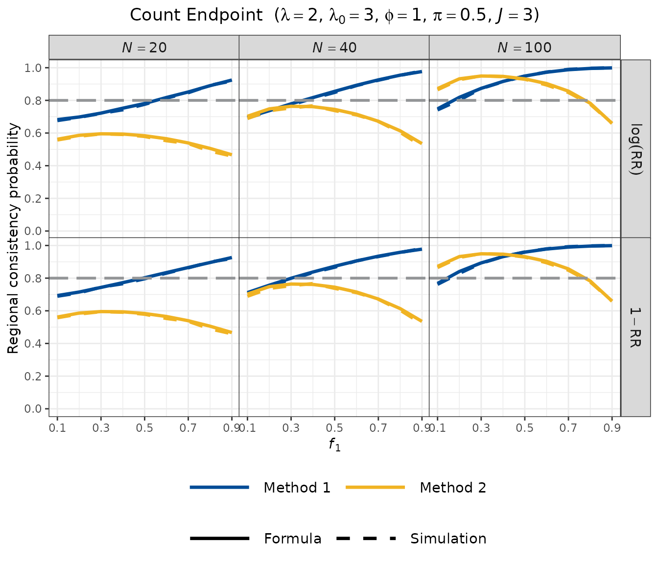
Setting: $\lambda = 2$, $\lambda_0 = 3$, $\phi = 1$, $N = 100$ ($J = 3$ regions with $N_1 = 20$), $\pi = 0.5$.

result_f <- rcp1armCount(
  lambda     = 2,
  lambda0    = 3,
  dispersion = 1,
  Nj         = c(20, 40, 40),
  PI         = 0.5,
  approach   = "formula"
)
print(result_f)
#> 
#> Regional Consistency Probability for Single-Arm MRCT
#> Endpoint : Count (Negative Binomial)
#> 
#>    Approach       : Exact Solution
#>    Expected Count : lambda     = 2.000000
#>    Control Count  : lambda0    = 3.000000
#>    Dispersion     : dispersion = 1.000000
#>    Sample Size    : Nj         = (20, 40, 40)
#>    Total Size     : N          = 100
#>    Threshold      : PI         = 0.5000
#> 
#> Consistency Probabilities:
#>    Method 1 (Region 1 vs Overall):
#>       Log-RR based    : 0.8186
#>       Linear-RR based : 0.8406
#>    Method 2 (All Regions Show Benefit):
#>       RR < 1          : 0.9320

result_s <- rcp1armCount(
  lambda     = 2,
  lambda0    = 3,
  dispersion = 1,
  Nj         = c(20, 40, 40),
  PI         = 0.5,
  approach   = "simulation",
  nsim       = 10000,
  seed       = 1
)
print(result_s)
#> 
#> Regional Consistency Probability for Single-Arm MRCT
#> Endpoint : Count (Negative Binomial)
#> 
#>    Approach       : Simulation-Based (nsim = 10000)
#>    Expected Count : lambda     = 2.000000
#>    Control Count  : lambda0    = 3.000000
#>    Dispersion     : dispersion = 1.000000
#>    Sample Size    : Nj         = (20, 40, 40)
#>    Total Size     : N          = 100
#>    Threshold      : PI         = 0.5000
#> 
#> Consistency Probabilities:
#>    Method 1 (Region 1 vs Overall):
#>       Log-RR based    : 0.8118
#>       Linear-RR based : 0.8331
#>    Method 2 (All Regions Show Benefit):
#>       RR < 1          : 0.9276

The output reports three RCP values: Method 1 on the log-RR scale (Method1_logRR), Method 1 on the linear-RR scale (Method1_linearRR), and Method 2 (Method2).

Visualisation

The count endpoint plot uses a grid layout: facet rows distinguish the two Method 1 scales (log-RR and $1 - RR$), and facet columns correspond to different total sample sizes.

plot_rcp1armCount(
  lambda     = 2,
  lambda0    = 3,
  dispersion = 1,
  PI         = 0.5,
  N_vec      = c(20, 40, 100),
  J          = 3,
  nsim       = 5000,
  seed       = 1,
  base_size  = 11
)

---

Summary

Endpoint	Model	Effect parameter	Benefit direction	Method 1 computation	Method 2 computation
Continuous	Normal	$\delta = \mu - \mu_0$	$\hat{\mu}_j > \mu_0$	Closed-form (normal approximation)	Product of normal tail probabilities
Binary	Binomial	$\delta = p - p_0$	$\hat{p}_j > p_0$	Exact enumeration (binomial)	Product of binomial tail probabilities
Count	Negative binomial	$\log(RR) = \log(\lambda/\lambda_0)$ (Method 1, log-RR scale); $1 - RR = 1 - \lambda/\lambda_0$ (Method 1, linear-RR scale)	$\widehat{RR}_j < 1$	Exact enumeration (negative binomial)	Product of NB tail probabilities

---

References

Homma G (2024). Cautionary note on regional consistency evaluation in multiregional clinical trials with binary outcomes. Pharmaceutical Statistics, 23(3):385–398. https://doi.org/10.1002/pst.2358