Plot Regional Consistency Probability for Single-Arm MRCT (Binary Endpoint)

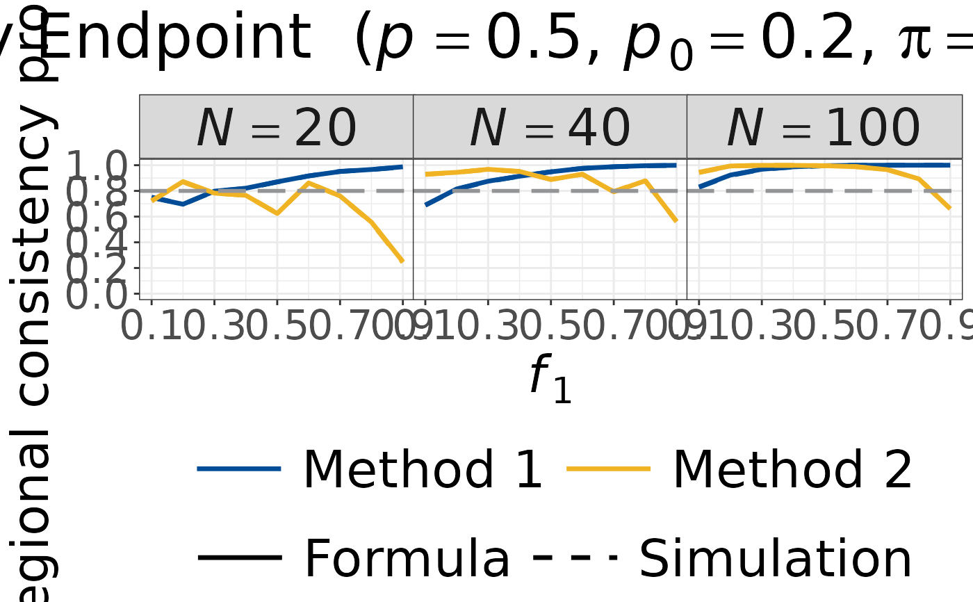
Generate a faceted plot of Regional Consistency Probability (RCP) as a function of the regional allocation proportion \(f_1\) for binary endpoints. Formula and simulation results are shown together for both Method 1 and Method 2. Facet columns correspond to total sample sizes specified in N_vec.

Regional sample sizes are allocated as: \(N_{j1} = \lfloor N \times f_1 \rfloor\) and \(N_{j2} = \cdots = N_{jJ} = (N - N_{j1}) / (J - 1)\).

Usage

plot_rcp1armBinary(
  p = 0.5,
  p0 = 0.2,
  PI = 0.5,
  N_vec = c(20, 40, 100),
  J = 3,
  f1_seq = seq(0.1, 0.9, by = 0.1),
  nsim = 10000,
  seed = 1,
  base_size = 28
)

Arguments

p

Numeric scalar. True response rate under the alternative hypothesis. Must be in \((0, 1)\). Default is 0.5.

p0

Numeric scalar. Null hypothesis response rate. Must be in \([0, 1)\). Default is 0.2.

PI

Numeric scalar. Effect retention threshold for Method 1. Must be in \([0, 1]\). Default is 0.5.

N_vec

Integer vector. Total sample sizes for each facet column. Default is c(20, 40, 100).

J

Positive integer (>= 2). Number of regions. Default is 3.

f1_seq

Numeric vector. Sequence of Region 1 allocation proportions. Each value must be in \((0, 1)\). Default is seq(0.1, 0.9, by = 0.1).

nsim

Positive integer. Number of Monte Carlo iterations for simulation. Default is 10000.

seed

Non-negative integer. Random seed for simulation. Default is 1.

base_size

Positive numeric. Base font size in points passed to theme. Use larger values (e.g., 28) for presentation slides and smaller values (e.g., 11) for vignettes or reports. Default is 28.

Value

A ggplot2 object.

Examples

p <- plot_rcp1armBinary(
  p     = 0.5,
  p0    = 0.2,
  PI    = 0.5,
  N_vec = c(20, 40, 100),
  J     = 3
)
print(p)