Mixed Count and Continuous Co-Primary Endpoints

Overview

This vignette demonstrates sample size calculation and power analysis for clinical trials with two co-primary endpoints: an overdispersed count outcome (following negative binomial distribution) and a continuous outcome (following normal distribution). The methodology is based on Homma and Yoshida (2024).

library(twoCoprimary)
library(dplyr)
library(tidyr)
library(knitr)

Background

Clinical Context

In clinical trials for treating asthma and chronic obstructive pulmonary disease (COPD), regulatory agencies require evaluation of both:

1. Count endpoint: Number of exacerbations over follow-up period (overdispersed count data)
2. Continuous endpoint: Lung function measure such as $\text{FEV}_{1}$ (forced expiratory volume in 1 second)

Why Negative Binomial Distribution?

Count outcomes in clinical trials often exhibit overdispersion, where the variance substantially exceeds the mean. The Poisson distribution assumes variance = mean, which is often violated.

Negative binomial (NB) distribution accommodates overdispersion:

$$X \sim \text{NB}(\lambda, \nu)$$

• Mean: $\text{E}[X] = \lambda = r \times t$ (rate $\times$ time)
• Variance: $\text{Var}[X] = \lambda + \lambda^{2}/\nu$
• Dispersion parameter: $\nu > 0$ controls overdispersion
  • As $\nu \to \infty$: $\text{NB} \to \text{Poisson}$ (no overdispersion)
  • Small $\nu$: High overdispersion (variance $\gg$ mean)

Variance-to-mean ratio (VMR): $$\text{VMR} = \frac{\text{Var}[X]}{\text{E}[X]} = 1 + \frac{\lambda}{\nu}$$

When $\text{VMR} > 1$, data are overdispersed and NB is more appropriate than Poisson.

Statistical Framework

Model and Assumptions

Consider a two-arm superiority trial with sample sizes $n_{1}$ (treatment) and $n_{2}$ (control), with allocation ratio $r = n_{1}/n_{2}$.

For subject $i$ in group $j$ ($j = 1$: treatment, $j = 2$: control), we observe two outcomes:

Outcome 1 (Count): $$X_{i,j,1} \sim \text{NB}(\lambda_{j}, \nu)$$

where $\lambda_{j}$ is the expected number of events in group $j$, and $\nu > 0$ is the common dispersion parameter.

Outcome 2 (Continuous): $$X_{i,j,2} \sim \text{N}(\mu_{j}, \sigma^{2})$$

where $\mu_{j}$ is the population mean in group $j$, and $\sigma^{2}$ is the common variance across groups.

Correlation Structure

The correlation between count and continuous outcomes within subjects is measured by $\rho_{j}$ in group $j$. This correlation must satisfy feasibility constraints based on the Fréchet-Hoeffding copula bounds, which depend on the marginal distributions.

Use the corrbound2MixedCountContinuous() function to check valid correlation bounds for given parameters.

Hypothesis Testing

We test superiority of treatment over control for both endpoints. Note: In COPD/asthma trials, treatment benefit is indicated by lower values for both endpoints (fewer exacerbations, less decline in lung function).

For count endpoint (1): $$\text{H}_{01}: r_{1} \geq r_{2} \text{ vs. } \text{H}_{11}: r_{1} < r_{2}$$

Equivalently, testing $\beta_{1} = \log(r_{1}) - \log(r_{2}) < 0$.

For continuous endpoint (2): $$\text{H}_{02}: \mu_{1} - \mu_{2} \geq 0 \text{ vs. } \text{H}_{12}: \mu_{1} - \mu_{2} < 0$$

Co-primary endpoints (intersection-union test): $$\text{H}_0 = \text{H}_{01} \cup \text{H}_{02} \text{ vs. } \text{H}_1 = \text{H}_{11} \cap \text{H}_{12}$$

Reject $\text{H}_{0}$ at level $\alpha$ if and only if both $\text{H}_{01}$ and $\text{H}_{02}$ are rejected at level $\alpha$.

Test Statistics

Count endpoint (Equation 7 in Homma and Yoshida, 2024):

$$Z_{1} = \frac{\hat{\beta}_{1}}{\sqrt{\text{Var}(\hat{\beta}_{1})}}$$

where:

• $\hat{\beta}_{1} = \log(\bar{X}_{1,1}) - \log(\bar{X}_{2,1})$ is the log rate ratio
• $\text{Var}(\hat{\beta}_{1}) = \frac{1}{n_{2}}\left[\frac{1}{t}\left(\frac{1}{\lambda_{2}} + \frac{1}{r\lambda_{1}}\right) + \frac{1+r}{\nu r}\right] = \frac{V_{a}}{n_{2}}$

Continuous endpoint:

$$Z_{2} = \frac{\bar{X}_{1,2} - \bar{X}_{2,2}}{\sigma\sqrt{\frac{1+r}{r n_{2}}}}$$

When $\sigma$ is a common known standard deviation.

Joint Distribution and Correlation

Under $\text{H}_{1}$, the test statistics $(Z_{1}, Z_{2})$ asymptotically follow a bivariate normal distribution (Appendix B in Homma and Yoshida, 2024):

$$\begin{pmatrix} Z_1 \\ Z_2 \end{pmatrix} \sim \text{BN}\left(\begin{pmatrix} \omega_1 \\ \omega_2 \end{pmatrix}, \begin{pmatrix} 1 & \gamma \\ \gamma & 1 \end{pmatrix}\right)$$

where:

• $\omega_{1} = \frac{\sqrt{n_{2}}\beta_{1}}{\sqrt{V_{a}}}$ with $\beta_{1} = \log(r_{1}) - \log(r_{2})$
• $\omega_{2} = \frac{\delta}{\sigma\sqrt{\frac{1+r}{r n_{2}}}}$ with $\delta = \mu_{1} - \mu_{2}$

Correlation between test statistics (Equation 11 in Homma and Yoshida, 2024):

$$\gamma = \sum_{j=1}^{2} \frac{n_{2}\rho_{j}\sqrt{1+\lambda_{j}/\nu}}{n_{j}\sqrt{\lambda_{j}V_{a}(1+r)/r}}$$

For balanced design ($r = 1$) with common correlation ($\rho_{1} = \rho_{2} = \rho$):

$$\gamma = \frac{\rho}{\sqrt{2}}\frac{\sqrt{1/\lambda_{2} + 1/\nu} + \sqrt{1/\lambda_{1} + 1/\nu}}{\sqrt{(1/\lambda_{2} + 1/\lambda_{1} + 2/\nu)}}$$

Power Calculation

The overall power is (Equation 10 in Homma and Yoshida, 2024):

$$1 - \beta = \text{P}(Z_{1} < z_{\alpha} \cap Z_{2} < z_{\alpha} \mid \text{H}_{1})$$

Using the bivariate normal CDF $\Phi_{2}$:

$$1 - \beta = \Phi_{2}\left(z_{\alpha} - \frac{\sqrt{n_{2}}(\log r_{1} - \log r_{2})}{\sqrt{V_{a}}}, z_{\alpha} - \frac{\sqrt{n_{2}}(\mu_{1}-\mu_{2})}{\sigma\sqrt{\frac{1+r}{r}}} \Bigg| \gamma\right)$$

Sample Size Determination

The sample size is determined by solving the power equation numerically. For a given allocation ratio $r$, target power $1 - \beta$, and significance level $\alpha$, we find the smallest $n_{2}$ such that the overall power equals or exceeds $1 - \beta$.

Sequential search algorithm:

1. Calculate initial sample size based on single-endpoint formulas
2. Compute power at current sample size
3. If power $\geq$ target: decrease $n_{2}$ until power $<$ target, then add 1 back
4. If power $<$ target: increase $n_{2}$ until power $\geq$ target

Correlation Bounds

Example: Calculate Correlation Bounds

# Scenario: lambda = 1.25, nu = 0.8, mu = 0, sigma = 250
bounds1 <- corrbound2MixedCountContinuous(lambda = 1.25, nu = 0.8, mu = 0, sd = 250)
cat("Correlation bounds for NB(1.25, 0.8) and N(0, 250²):\n")
#> Correlation bounds for NB(1.25, 0.8) and N(0, 250²):
cat("Lower bound:", round(bounds1[1], 3), "\n")
#> Lower bound: -0.846
cat("Upper bound:", round(bounds1[2], 3), "\n\n")
#> Upper bound: 0.846

# Higher dispersion (smaller nu) typically restricts bounds
bounds2 <- corrbound2MixedCountContinuous(lambda = 1.25, nu = 0.5, mu = 0, sd = 250)
cat("Correlation bounds for NB(1.25, 0.5) and N(0, 250²):\n")
#> Correlation bounds for NB(1.25, 0.5) and N(0, 250²):
cat("Lower bound:", round(bounds2[1], 3), "\n")
#> Lower bound: -0.802
cat("Upper bound:", round(bounds2[2], 3), "\n\n")
#> Upper bound: 0.802

# Higher mean count
bounds3 <- corrbound2MixedCountContinuous(lambda = 2.0, nu = 0.8, mu = 0, sd = 250)
cat("Correlation bounds for NB(2.0, 0.8) and N(0, 250²):\n")
#> Correlation bounds for NB(2.0, 0.8) and N(0, 250²):
cat("Lower bound:", round(bounds3[1], 3), "\n")
#> Lower bound: -0.863
cat("Upper bound:", round(bounds3[2], 3), "\n")
#> Upper bound: 0.863

Important: Always verify that the specified correlation $\rho$ is within the feasible bounds for your parameters.

Replicating Homma and Yoshida (2024) Table 1 (Case B)

Table 1 from Homma and Yoshida (2024) shows sample sizes and operating characteristics for various scenarios. We replicate Case B with $\nu = 3$ and $\nu = 5$.

Design parameters for Case B:

• Count rates: $r_{2} = 1$, $r_{1} = 2$, $t = 1$ → $\lambda_{2} = 1$, $\lambda_{1} = 2$
• Dispersion: $\nu = 3$ and $5$
• Continuous means: $\mu_{2} = 0$, $\mu_{1} = -50$ (negative indicates less decline)
• Standard deviation: $\sigma = 75$
• $\alpha = 0.025$ (one-sided), $1 - \beta = 0.9$ (target power)
• Balanced allocation: $r = 1$ ($n_{1} = n_{2}$)

# Define scenarios for Table 1 Case B
scenarios_table1_B <- expand.grid(
  nu = c(3, 5),
  rho = c(0, 0.2, 0.4, 0.6, 0.8),
  stringsAsFactors = FALSE
)

# Calculate sample sizes for each scenario
results_table1_B <- lapply(1:nrow(scenarios_table1_B), function(i) {
  nu_val <- scenarios_table1_B$nu[i]
  rho_val <- scenarios_table1_B$rho[i]
  
  result <- ss2MixedCountContinuous(
    r1 = 1,
    r2 = 2,
    nu = nu_val,
    t = 1,
    mu1 = -50,
    mu2 = 0,
    sd = 75,
    r = 1,
    rho1 = rho_val,
    rho2 = rho_val,
    alpha = 0.025,
    beta = 0.1
  )
  
  data.frame(
    nu = nu_val,
    rho = rho_val,
    n2 = result$n2,
    n1 = result$n1,
    N = result$N
  )
})

table1_B_results <- bind_rows(results_table1_B)

# Display results grouped by nu
table1_B_nu3 <- table1_B_results %>%
  filter(nu == 3) %>%
  select(rho, n2, N)

table1_B_nu5 <- table1_B_results %>%
  filter(nu == 5) %>%
  select(rho, n2, N)

kable(table1_B_nu3, 
      caption = "Table 1 Case B: Sample Sizes (ν = 3, Balanced Design, α = 0.025, 1-β = 0.9)",
      digits = 1,
      col.names = c("ρ", "n per group", "N total"))

Table 1 Case B: Sample Sizes (ν = 3, Balanced Design, α = 0.025, 1-β = 0.9)

ρ	n per group	N total
0.0	59	118
0.2	58	116
0.4	57	114
0.6	56	112
0.8	54	108

kable(table1_B_nu5, 
      caption = "Table 1 Case B: Sample Sizes (ν = 5, Balanced Design, α = 0.025, 1-β = 0.9)",
      digits = 1,
      col.names = c("ρ", "n per group", "N total"))

Table 1 Case B: Sample Sizes (ν = 5, Balanced Design, α = 0.025, 1-β = 0.9)

ρ	n per group	N total
0.0	55	110
0.2	55	110
0.4	54	108
0.6	53	106
0.8	51	102

Observations:

• Higher dispersion parameter $\nu$ (less overdispersion) requires smaller sample sizes
• Correlation reduces sample size: approximately 2-4% at $\rho = 0.4$, 5-8% at $\rho = 0.8$
• The effect of correlation is moderate compared to other endpoint combinations

Basic Usage Examples

Example 1: Balanced Design

Calculate sample size for a balanced design with moderate effect sizes:

# Balanced design: n1 = n2 (i.e., r = 1)
result_balanced <- ss2MixedCountContinuous(
  r1 = 1.0,              # Count rate in treatment group
  r2 = 1.25,             # Count rate in control group
  nu = 0.8,              # Dispersion parameter
  t = 1,                 # Follow-up time
  mu1 = -50,             # Mean for treatment (negative = benefit)
  mu2 = 0,               # Mean for control
  sd = 250,              # Standard deviation
  r = 1,                 # Balanced allocation
  rho1 = 0.5,            # Correlation in treatment group
  rho2 = 0.5,            # Correlation in control group
  alpha = 0.025,
  beta = 0.2
)

print(result_balanced)
#> 
#> Sample size calculation for mixed count and continuous co-primary endpoints
#> 
#>              n1 = 705
#>              n2 = 705
#>               N = 1410
#>              sd = 250
#>            rate = 1, 1.25
#>              nu = 0.8
#>               t = 1
#>              mu = -50, 0
#>             rho = 0.5, 0.5
#>      allocation = 1
#>           alpha = 0.025
#>            beta = 0.2

Example 2: Effect of Correlation

Demonstrate how correlation affects sample size:

# Fixed effect sizes
r1 <- 1.0
r2 <- 1.25
nu <- 0.8
mu1 <- -50
mu2 <- 0
sd <- 250

# Range of correlations
rho_values <- c(0, 0.2, 0.4, 0.6, 0.8)

ss_by_rho <- sapply(rho_values, function(rho) {
  result <- ss2MixedCountContinuous(
    r1 = r1, r2 = r2, nu = nu, t = 1,
    mu1 = mu1, mu2 = mu2, sd = sd,
    r = 1,
    rho1 = rho, rho2 = rho,
    alpha = 0.025,
    beta = 0.2
  )
  result$n2
})

result_df <- data.frame(
  rho = rho_values,
  n_per_group = ss_by_rho,
  N_total = ss_by_rho * 2,
  reduction_pct = round((1 - ss_by_rho / ss_by_rho[1]) * 100, 1)
)

kable(result_df,
      caption = "Effect of Correlation on Sample Size",
      col.names = c("ρ", "n per group", "N total", "Reduction (%)"))

Effect of Correlation on Sample Size

ρ	n per group	N total	Reduction (%)
0.0	727	1454	0.0
0.2	720	1440	1.0
0.4	711	1422	2.2
0.6	699	1398	3.9
0.8	685	1370	5.8

# Plot
plot(rho_values, ss_by_rho, 
     type = "b", pch = 19,
     xlab = "Correlation (ρ)", 
     ylab = "Sample size per group (n)",
     main = "Effect of Correlation on Sample Size",
     ylim = c(600, max(ss_by_rho) * 1.1))
grid()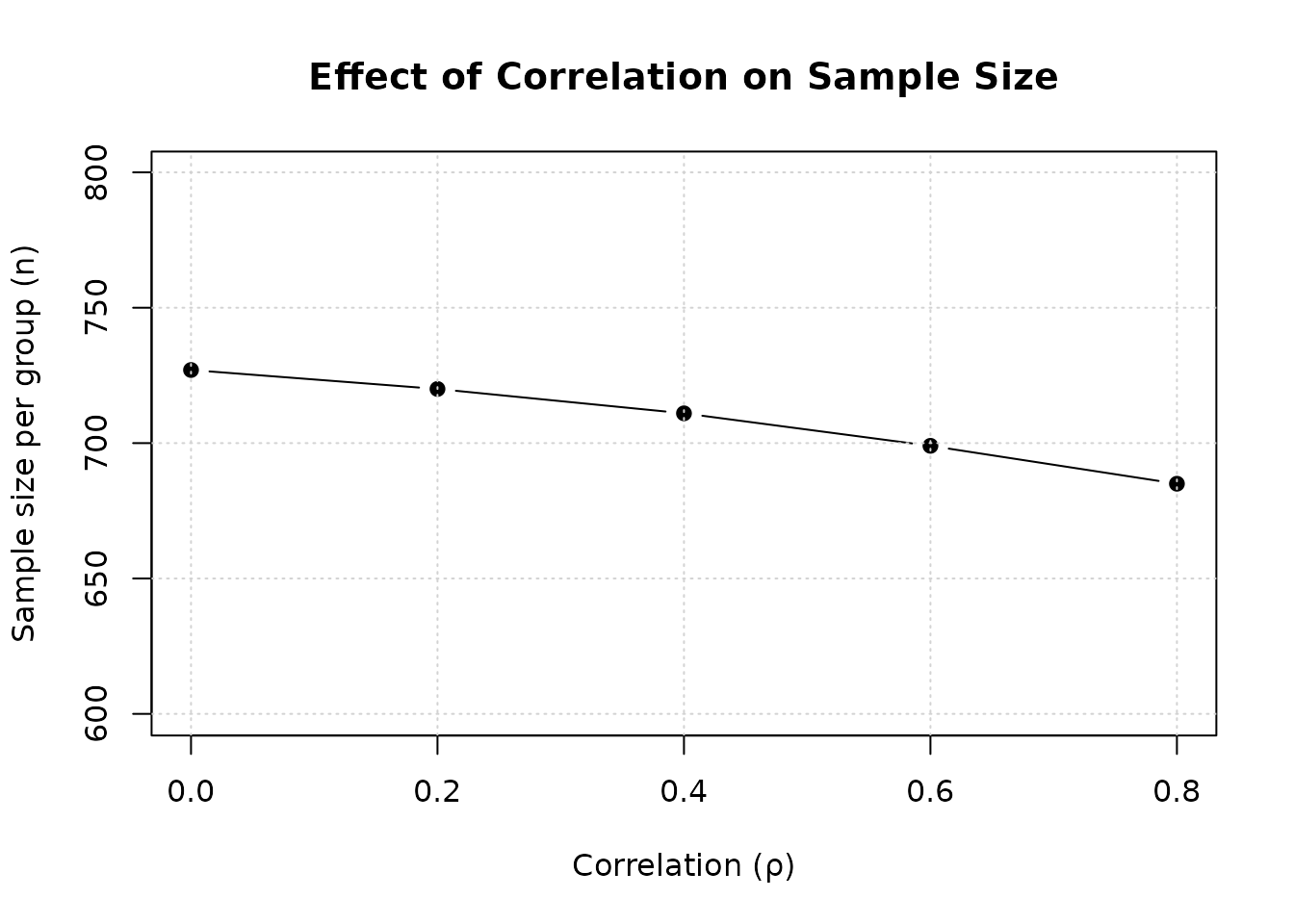

Interpretation: Higher positive correlation reduces required sample size. At $\rho = 0.8$, sample size is reduced by approximately 5-7% compared to $\rho = 0$.

Example 3: Effect of Dispersion Parameter

Compare sample sizes for different levels of overdispersion:

# Fixed design parameters
r1 <- 1.0
r2 <- 1.25
mu1 <- -50
mu2 <- 0
sd <- 250
rho <- 0.5

# Range of dispersion parameters
nu_values <- c(0.5, 0.8, 1.0, 2.0, 5.0)

ss_by_nu <- sapply(nu_values, function(nu) {
  result <- ss2MixedCountContinuous(
    r1 = r1, r2 = r2, nu = nu, t = 1,
    mu1 = mu1, mu2 = mu2, sd = sd,
    r = 1,
    rho1 = rho, rho2 = rho,
    alpha = 0.025,
    beta = 0.2
  )
  result$n2
})

result_df_nu <- data.frame(
  nu = nu_values,
  VMR = round(1 + 1.125/nu_values, 2),  # VMR at lambda = 1.125 (average)
  n_per_group = ss_by_nu,
  N_total = ss_by_nu * 2
)

kable(result_df_nu,
      caption = "Effect of Dispersion Parameter on Sample Size",
      digits = c(1, 2, 0, 0),
      col.names = c("ν", "VMR", "n per group", "N total"))

Effect of Dispersion Parameter on Sample Size

ν	VMR	n per group	N total
0.5	3.25	921	1842
0.8	2.41	705	1410
1.0	2.12	639	1278
2.0	1.56	522	1044
5.0	1.23	463	926

Key finding: Higher overdispersion (smaller $\nu$, larger VMR) requires larger sample sizes.

Example 4: Unbalanced Allocation

Calculate sample size with 2:1 allocation ratio:

# Balanced design (r = 1)
result_balanced <- ss2MixedCountContinuous(
  r1 = 1.0, r2 = 1.25, nu = 0.8, t = 1,
  mu1 = -50, mu2 = 0, sd = 250,
  r = 1,
  rho1 = 0.5, rho2 = 0.5,
  alpha = 0.025,
  beta = 0.2
)

# Unbalanced design (r = 2, i.e., n1 = 2*n2)
result_unbalanced <- ss2MixedCountContinuous(
  r1 = 1.0, r2 = 1.25, nu = 0.8, t = 1,
  mu1 = -50, mu2 = 0, sd = 250,
  r = 2,
  rho1 = 0.5, rho2 = 0.5,
  alpha = 0.025,
  beta = 0.2
)

comparison_allocation <- data.frame(
  Design = c("Balanced (1:1)", "Unbalanced (2:1)"),
  n_treatment = c(result_balanced$n1, result_unbalanced$n1),
  n_control = c(result_balanced$n2, result_unbalanced$n2),
  N_total = c(result_balanced$N, result_unbalanced$N)
)

kable(comparison_allocation,
      caption = "Comparison: Balanced vs Unbalanced Allocation",
      col.names = c("Design", "n₁", "n₂", "N total"))

Comparison: Balanced vs Unbalanced Allocation

Design	n₁	n₂	N total
Balanced (1:1)	705	705	1410
Unbalanced (2:1)	1044	522	1566

cat("\nIncrease in total sample size:", 
    round((result_unbalanced$N - result_balanced$N) / result_balanced$N * 100, 1), "%\n")
#> 
#> Increase in total sample size: 11.1 %

Power Verification

Verify that calculated sample sizes achieve target power:

# Use result from Example 1
power_result <- power2MixedCountContinuous(
  n1 = result_balanced$n1,
  n2 = result_balanced$n2,
  r1 = 1.0,
  r2 = 1.25,
  nu = 0.8,
  t = 1,
  mu1 = -50,
  mu2 = 0,
  sd = 250,
  rho1 = 0.5,
  rho2 = 0.5,
  alpha = 0.025
)

cat("Target power: 0.80\n")
#> Target power: 0.80
cat("Achieved power (Count endpoint):", round(as.numeric(power_result$power1), 4), "\n")
#> Achieved power (Count endpoint):
cat("Achieved power (Continuous endpoint):", round(as.numeric(power_result$power2), 4), "\n")
#> Achieved power (Continuous endpoint):
cat("Achieved power (Co-primary):", round(as.numeric(power_result$powerCoprimary), 4), "\n")
#> Achieved power (Co-primary): 0.8003

Practical Recommendations

Design Considerations

1. Estimating dispersion parameter: Use pilot data or historical studies to estimate $\nu$. Underestimating $\nu$ (overestimating overdispersion) leads to conservative sample sizes.

2. Estimating correlation: Use pilot data; be conservative if uncertain ($\rho = 0$ is conservative).

3. Direction of benefit: For COPD/asthma trials, ensure test directions are correct (lower is better for both endpoints).

4. Balanced allocation: Generally most efficient ($r = 1$) unless practical constraints require otherwise.

5. Sensitivity analysis: Calculate sample sizes for range of plausible $\nu$, $\rho$, and effect sizes.

When to Use This Method

Use mixed count-continuous methods when:

• One endpoint is an overdispersed count (exacerbations, events)
• Other endpoint is continuous (lung function, quality of life)
• Both endpoints are clinically meaningful co-primary endpoints
• Negative binomial distribution is appropriate for count data

Challenges and Considerations

1. Overdispersion estimation: Requires historical data or pilot studies; misspecification affects sample size

2. Correlation estimation: Correlation between count and continuous outcomes is challenging to estimate

3. Direction specification: Ensure treatment benefit direction is correctly specified for both endpoints

References

Homma, G., & Yoshida, T. (2024). Sample size calculation in clinical trials with two co-primary endpoints including overdispersed count and continuous outcomes. Pharmaceutical Statistics, 23(1), 46-59.