Two Continuous Co-Primary Endpoints • twoCoprimary

Overview

This vignette demonstrates sample size calculation and power analysis for clinical trials with two co-primary continuous endpoints using asymptotic normal approximation methods. The methodology is based on Sozu et al. (2011).

library(twoCoprimary)
library(dplyr)
library(tidyr)
library(knitr)

Background and Motivation

What are Co-Primary Endpoints?

In clinical trials, co-primary endpoints require demonstrating statistically significant treatment effects on all endpoints simultaneously. Unlike multiple primary endpoints (where success on any one endpoint is sufficient), co-primary endpoints require:

Rejecting all null hypotheses at level $\alpha$
No multiplicity adjustment needed for Type I error control
Correlation consideration can improve efficiency

Clinical Examples

Co-primary continuous endpoints are common in:

Alzheimer’s disease trials: Cognitive function (ADAS-cog) + Clinical global impression (CIBIC-plus)
Irritable bowel syndrome (IBS) trials: Pain intensity and stool frequency of IBS with constipation (IBS-C) + Pain intensity and stool consistency of IBS with diarrhea (IBS-D)

Statistical Framework

Model and Assumptions

Consider a two-arm parallel-group superiority trial comparing treatment (group 1) with control (group 2). Let $n_{1}$ and $n_{2}$ denote the sample sizes in the two groups (i.e., total sample size is $N=n_{1}+n_{2}$ ), and define the allocation ratio $r = n_{1}/n_{2}$ .

For subject $i$ in group $j$ ( $j = 1$ : treatment, $j = 2$ : control), we observe two continuous outcomes:

Endpoint $k$ ( $k = 1, 2$ ): $X_{i,j,k} \sim \text{N}(\mu_{j,k}, \sigma_{k}^{2})$

where:

$\mu_{j,k}$ is the population mean for outcome $k$ in group $j$
$\sigma_{k}^{2}$ is the common variance for outcome $k$ across both groups

Within-subject correlation: The two outcomes are correlated within each subject: $\text{Cor}(X_{i,j,1}, X_{i,j,2}) = \rho_{j}$

We assume common correlation across groups: $\rho_{1} = \rho_{2} = \rho$ .

Effect Size Parameterization

The treatment effect for endpoint $k$ is measured by:

Absolute difference: $\delta_{k} = \mu_{1,k} - \mu_{2,k}$

Standardized effect size: $\delta_{k}^{\ast} = \delta_{k} / \sigma_{k}$

The standardized effect size is preferred as it is scale-free and facilitates comparison across studies.

Hypothesis Testing

For two co-primary endpoints, we test:

Null hypothesis: $\text{H}_{0} = \text{H}_{01} \cup \text{H}_{02}$ (at least one null hypothesis is true)

where $\text{H}_{0k}: \delta_{k} = 0$ for $k = 1, 2$ .

Alternative hypothesis: $\text{H}_{1} = \text{H}_{11} \cap \text{H}_{12}$ (both alternative hypotheses are true)

where $\text{H}_{1k}: \delta_{k} > 0$ for $k = 1, 2$ .

Decision rule: Reject $\text{H}_{0}$ if and only if both $\text{H}_{01}$ and $\text{H}_{02}$ are rejected at significance level $\alpha$ .

Test Statistics

For each endpoint $k$ , the test statistic is:

Known variance case: $Z_{k} = \frac{\bar{X}_{1k} - \bar{X}_{2k}}{\sigma_{k}\sqrt{\frac{1}{n_{1}} + \frac{1}{n_{2}}}}$

Unknown variance case: $T_{k} = \frac{\bar{X}_{1k} - \bar{X}_{2k}}{s_{k}\sqrt{\frac{1}{n_{1}} + \frac{1}{n_{2}}}}$

where $s_{k}$ is the pooled sample standard deviation for endpoint $k$ .

Joint Distribution

Under $\text{H}_{1}$ , when variances are known, $(Z_{1}, Z_{2})$ asymptotically follows a bivariate normal distribution:

$\begin{pmatrix} Z_{1} \\ Z_{2} \end{pmatrix} \sim \text{BN}\left(\begin{pmatrix} \omega_{1} \\ \omega_{2} \end{pmatrix}, \begin{pmatrix} 1 & \gamma \\ \gamma & 1 \end{pmatrix}\right)$

where:

$\omega_{k} = \delta_{k}\sqrt{\frac{r n_{2}}{1 + r}}$ is the non-centrality parameter for endpoint $k$
$\gamma = \rho$ is the correlation between test statistics

Power Formula

The overall power is:

$1 - \beta = \Pr(Z_{1} > z_{1-\alpha} \text{ and } Z_{2} > z_{1-\alpha} \mid \text{H}_{1})$

Using the bivariate normal CDF:

$1 - \beta = \Phi_{2}(-z_{1-\alpha} + \omega_{1}, -z_{1-\alpha} + \omega_{2} \mid \rho)$

where $\Phi_{2}(\cdot, \cdot \mid \rho)$ is the bivariate normal CDF with correlation $\rho$ .

Sample Size Calculation

Basic Example

Calculate sample size for a balanced design ( $\kappa = 1$ ) with known variance:

# Design parameters
result <- ss2Continuous(
  delta1 = 0.5,      # Effect size for endpoint 1
  delta2 = 0.5,      # Effect size for endpoint 2
  sd1 = 1,           # Standard deviation for endpoint 1
  sd2 = 1,           # Standard deviation for endpoint 2
  rho = 0.5,         # Correlation between endpoints
  r = 1,             # Balanced allocation
  alpha = 0.025,     # One-sided significance level
  beta = 0.2,        # Type II error (80% power)
  known_var = TRUE
)

print(result)
#> 
#> Sample size calculation for two continuous co-primary endpoints
#> 
#>              n1 = 79
#>              n2 = 79
#>               N = 158
#>           delta = 0.5, 0.5
#>              sd = 1, 1
#>             rho = 0.5
#>      allocation = 1
#>           alpha = 0.025
#>            beta = 0.2
#>       known_var = TRUE

Impact of Correlation

Examine how correlation affects sample size:

# Calculate sample sizes for different correlations
correlations <- c(0, 0.3, 0.5, 0.8)
sample_sizes <- sapply(correlations, function(rho) {
  ss2Continuous(
    delta1 = 0.5, delta2 = 0.5,
    sd1 = 1, sd2 = 1,
    rho = rho, r = 1,
    alpha = 0.025, beta = 0.2,
    known_var = TRUE
  )$N
})

# Create summary table
correlation_table <- data.frame(
  Correlation = correlations,
  Total_N = sample_sizes,
  Reduction = c(0, round((1 - sample_sizes[-1]/sample_sizes[1]) * 100, 1))
)

kable(correlation_table,
      caption = "Sample Size vs Correlation (delta = 0.5, alpha = 0.025, power = 0.8)",
      col.names = c("Correlation (rho)", "Total N", "Reduction (%)"))

Sample Size vs Correlation (delta = 0.5, alpha = 0.025, power = 0.8)
Correlation (rho)	Total N	Reduction (%)
0.0	166	0.0
0.3	162	2.4
0.5	158	4.8
0.8	148	10.8

Key finding: At $\rho = 0.8$ , approximately 11% reduction in sample size compared to $\rho = 0$ .

Visualization with plot()

Visualize the relationship between correlation and sample size:

# Use plot method to visualize sample size vs correlation
plot(result, type = "sample_size_rho")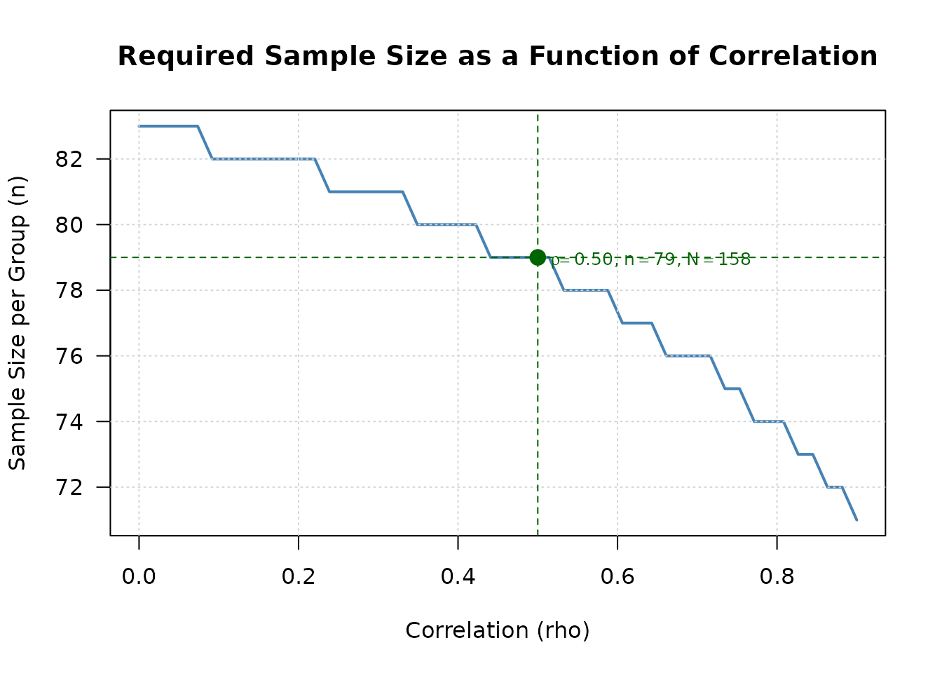

Visualize power contours for different effect sizes:

# Create contour plot for effect sizes
plot(result, type = "effect_contour")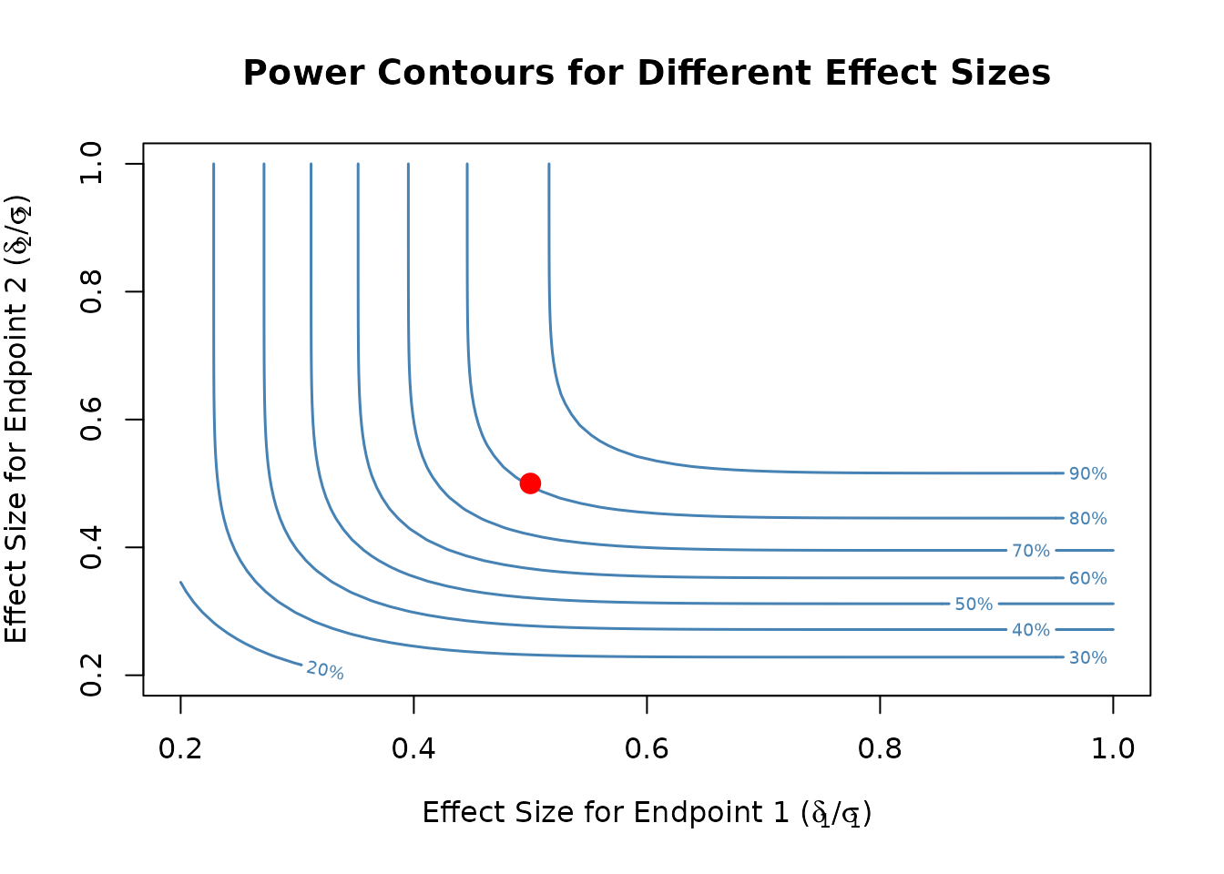

Replicating Sozu et al. (2011) Table 1

We replicate Table 1 from Sozu et al. (2011) using the design_table() function. This table shows sample sizes per group for various combinations of standardized effect sizes.

# Create parameter grid (delta1 <= delta2)
param_grid <- expand.grid(
  delta1 = c(0.2, 0.25, 0.3, 0.35, 0.4),
  delta2 = c(0.2, 0.25, 0.3, 0.35, 0.4),
  sd1 = 1,
  sd2 = 1
) %>% 
  arrange(delta1, delta2) %>% 
  filter(delta2 >= delta1)

# Calculate sample sizes for different correlations
result_table <- design_table(
  param_grid = param_grid,
  rho_values = c(0, 0.3, 0.5, 0.8),
  r = 1,
  alpha = 0.025,
  beta = 0.2,
  endpoint_type = "continuous"
) %>% 
  mutate_at(vars(starts_with("rho_")), ~ . / 2)  # Per-group sample size

# Display table
kable(result_table,
      caption = "Table 1: Sample Sizes Per Group (Sozu et al. 2011, alpha = 0.025, power = 0.8)",
      digits = 2)

Table 1: Sample Sizes Per Group (Sozu et al. 2011, alpha = 0.025, power = 0.8)
delta1	delta2	sd1	sd2	rho_0.0	rho_0.3	rho_0.5	rho_0.8
0.20	0.20	1	1	516	503	490	458
0.20	0.25	1	1	432	424	417	401
0.20	0.30	1	1	402	399	397	393
0.20	0.35	1	1	394	394	393	393
0.20	0.40	1	1	393	393	393	393
0.25	0.25	1	1	330	322	314	294
0.25	0.30	1	1	284	278	272	260
0.25	0.35	1	1	263	260	257	253
0.25	0.40	1	1	254	253	253	252
0.30	0.30	1	1	230	224	218	204
0.30	0.35	1	1	201	197	192	183
0.30	0.40	1	1	186	183	181	176
0.35	0.35	1	1	169	165	160	150
0.35	0.40	1	1	150	147	143	136
0.40	0.40	1	1	129	126	123	115

Interpretation:

Each row represents a combination of standardized effect sizes ( $\delta_{1}^{\ast}, \delta_{2}^{\ast}$ )
Columns show sample size per group for different correlations ( $\rho = 0, 0.3, 0.5, 0.8$ )
Higher correlation leads to smaller required sample sizes
When $\delta_{1} = \delta_{2}$ (equal effect sizes), the benefit of correlation is more pronounced

Power Calculation

Power for a Given Sample Size

Calculate power for a specific sample size:

# Calculate power with n1 = n2 = 100
power_result <- power2Continuous(
  n1 = 100, n2 = 100,
  delta1 = 0.5, delta2 = 0.5,
  sd1 = 1, sd2 = 1,
  rho = 0.5,
  alpha = 0.025,
  known_var = TRUE
)

print(power_result)
#> 
#> Power calculation for two continuous co-primary endpoints
#> 
#>              n1 = 100
#>              n2 = 100
#>           delta = 0.5, 0.5
#>              sd = 1, 1
#>             rho = 0.5
#>           alpha = 0.025
#>       known_var = TRUE
#>          power1 = 0.942438
#>          power2 = 0.942438
#>  powerCoprimary = 0.899732

Power Verification

Verify that calculated sample size achieves target power:

# Calculate sample size
ss_result <- ss2Continuous(
  delta1 = 0.5, delta2 = 0.5,
  sd1 = 1, sd2 = 1,
  rho = 0.5, r = 1,
  alpha = 0.025, beta = 0.2,
  known_var = TRUE
)

# Verify power with calculated sample size
power_check <- power2Continuous(
  n1 = ss_result$n1, n2 = ss_result$n2,
  delta1 = 0.5, delta2 = 0.5,
  sd1 = 1, sd2 = 1,
  rho = 0.5,
  alpha = 0.025,
  known_var = TRUE
)

cat("Calculated sample size per group:", ss_result$n2, "\n")
#> Calculated sample size per group: 79
cat("Target power: 0.80\n")
#> Target power: 0.80
cat("Achieved power:", round(power_check$powerCoprimary, 4), "\n")
#> Achieved power: 0.8042

Unified Interface

The package provides a unified interface similar to power.prop.test():

# Sample size calculation mode
twoCoprimary2Continuous(
  delta1 = 0.5, delta2 = 0.5,
  sd1 = 1, sd2 = 1,
  rho = 0.5, power = 0.8, r = 1,
  alpha = 0.025, known_var = TRUE
)
#> 
#> Sample size calculation for two continuous co-primary endpoints
#> 
#>              n1 = 79
#>              n2 = 79
#>               N = 158
#>           delta = 0.5, 0.5
#>              sd = 1, 1
#>             rho = 0.5
#>      allocation = 1
#>           alpha = 0.025
#>            beta = 0.2
#>       known_var = TRUE

# Power calculation mode
twoCoprimary2Continuous(
  n1 = 100, n2 = 100,
  delta1 = 0.5, delta2 = 0.5,
  sd1 = 1, sd2 = 1,
  rho = 0.5,
  alpha = 0.025, known_var = TRUE
)
#> 
#> Power calculation for two continuous co-primary endpoints
#> 
#>              n1 = 100
#>              n2 = 100
#>           delta = 0.5, 0.5
#>              sd = 1, 1
#>             rho = 0.5
#>           alpha = 0.025
#>       known_var = TRUE
#>          power1 = 0.942438
#>          power2 = 0.942438
#>  powerCoprimary = 0.899732

Unknown Variance Case

When variances are unknown, use $t$ -test with Monte Carlo simulation:

# Sample size calculation with unknown variance
ss_unknown <- ss2Continuous(
  delta1 = 0.5, delta2 = 0.5,
  sd1 = 1, sd2 = 1,
  rho = 0.5, r = 1,
  alpha = 0.025, beta = 0.2,
  known_var = FALSE,
  nMC = 10000  # Number of Monte Carlo simulations
)

print(ss_unknown)
#> 
#> Sample size calculation for two continuous co-primary endpoints
#> 
#>              n1 = 80
#>              n2 = 80
#>               N = 160
#>           delta = 0.5, 0.5
#>              sd = 1, 1
#>             rho = 0.5
#>      allocation = 1
#>           alpha = 0.025
#>            beta = 0.2
#>       known_var = FALSE
#>             nMC = 10000

Note: The unknown variance case requires more computation time due to Monte Carlo simulation.

Practical Considerations

Correlation Estimation

Methods to estimate correlation $\rho$ :

Pilot studies: Small preliminary studies
Historical data: Previous trials in the same disease area
Literature review: Published studies with similar endpoints
Expert opinion: Clinical judgment when data are unavailable

Conservative approach: Use lower correlation estimates to ensure adequate power.

Sensitivity Analysis

Always perform sensitivity analysis:

# Test robustness to correlation misspecification
assumed_rho <- 0.5
true_rhos <- c(0, 0.3, 0.5, 0.7, 0.9)

# Calculate sample size assuming rho = 0.5
ss_assumed <- ss2Continuous(
  delta1 = 0.5, delta2 = 0.5,
  sd1 = 1, sd2 = 1,
  rho = assumed_rho, r = 1,
  alpha = 0.025, beta = 0.2,
  known_var = TRUE
)

# Calculate achieved power under different true correlations
sensitivity_results <- data.frame(
  Assumed_rho = assumed_rho,
  True_rho = true_rhos,
  n_per_group = ss_assumed$n2,
  Achieved_power = sapply(true_rhos, function(true_rho) {
    power2Continuous(
      n1 = ss_assumed$n1, n2 = ss_assumed$n2,
      delta1 = 0.5, delta2 = 0.5,
      sd1 = 1, sd2 = 1,
      rho = true_rho,
      alpha = 0.025,
      known_var = TRUE
    )$powerCoprimary
  })
)

kable(sensitivity_results,
      caption = "Sensitivity Analysis: Impact of Correlation Misspecification",
      digits = 3,
      col.names = c("Assumed rho", "True rho", "n per group", "Achieved Power"))

Sensitivity Analysis: Impact of Correlation Misspecification
Assumed rho	True rho	n per group	Achieved Power
0.5	0.0	79	0.777
0.5	0.3	79	0.791
0.5	0.5	79	0.804
0.5	0.7	79	0.821
0.5	0.9	79	0.846

References

Sozu, T., Sugimoto, T., & Hamasaki, T. (2011). Sample size determination in superiority clinical trials with multiple co-primary correlated endpoints. Journal of Biopharmaceutical Statistics, 21(4), 650-668.