Single Binary Endpoint • BayesianQDM

Motivating Scenario

We use a hypothetical Phase IIa proof-of-concept (PoC) trial in moderate-to-severe rheumatoid arthritis (RA). The investigational drug is compared with placebo in a 1:1 randomised controlled trial with $n_t = n_c = 12$ patients per group.

Endpoint: ACR20 response rate (proportion of patients achieving $\ge 20\%$ improvement in ACR criteria).

Clinically meaningful thresholds (posterior probability):

Target Value (TV) = 0.20 (treatment–control difference)
Minimum Acceptable Value (MAV) = 0.05

Null hypothesis threshold (predictive probability): $\theta_{\mathrm{NULL}} = 0.10$ .

Decision thresholds: $\gamma_{\mathrm{go}} = 0.80$ (Go), $\gamma_{\mathrm{nogo}} = 0.20$ (NoGo).

Observed data (used in Sections 2–4): $y_t = 8$ responders out of $n_t = 12$ (treatment); $y_c = 3$ responders out of $n_c = 12$ (control).

1. Bayesian Model: Beta-Binomial Conjugate

1.1 Prior Distribution

Let $\pi_j$ denote the true response rate in group $j$ ( $j = t$ : treatment, $j = c$ : control). We model the number of responders as

$y_j \mid \pi_j \;\sim\; \mathrm{Binomial}(n_j,\, \pi_j),$

and place independent Beta priors on each rate:

$\pi_j \;\sim\; \mathrm{Beta}(a_j,\, b_j),$

where $a_j > 0$ and $b_j > 0$ are the shape parameters.

The Jeffreys prior corresponds to $a_j = b_j = 0.5$ , giving a weakly informative, symmetric prior on $(0, 1)$ . The uniform prior corresponds to $a_j = b_j = 1$ .

1.2 Posterior Distribution

By conjugacy of the Beta-Binomial model, the posterior after observing $y_j$ responders among $n_j$ patients is

$\pi_j \mid y_j \;\sim\; \mathrm{Beta}(a_j^*,\, b_j^*),$

where the posterior shape parameters are

$a_j^* = a_j + y_j, \qquad b_j^* = b_j + n_j - y_j.$

The posterior mean and variance are

$E[\pi_j \mid y_j] = \frac{a_j^*}{a_j^* + b_j^*}, \qquad \mathrm{Var}(\pi_j \mid y_j) = \frac{a_j^*\, b_j^*}{(a_j^* + b_j^*)^2\,(a_j^* + b_j^* + 1)}.$

1.3 Posterior of the Treatment Effect

The treatment effect is $\theta = \pi_t - \pi_c$ . Since the two groups are independent, $\theta \mid y_t, y_c$ follows the distribution of the difference of two independent Beta random variables:

$\pi_t \mid y_t \;\sim\; \mathrm{Beta}(a_t^*,\, b_t^*), \qquad \pi_c \mid y_c \;\sim\; \mathrm{Beta}(a_c^*,\, b_c^*).$

There is no closed-form CDF for $\theta = \pi_t - \pi_c$ , so the posterior probability

$P(\theta > \theta_0 \mid y_t, y_c) = P(\pi_t - \pi_c > \theta_0 \mid y_t, y_c)$

is evaluated by the convolution integral implemented in pbetadiff():

$P(\pi_t - \pi_c > \theta_0) = \int_0^1 F_{\mathrm{Beta}(a_c^*, b_c^*)}\!\left(x - \theta_0\right)\, f_{\mathrm{Beta}(a_t^*, b_t^*)}\!(x)\; dx,$

where $F_{\mathrm{Beta}(\alpha,\beta)}$ is the Beta CDF and $f_{\mathrm{Beta}(\alpha,\beta)}$ is the Beta PDF. This one-dimensional integral is evaluated by adaptive Gauss-Kronrod quadrature via stats::integrate().

2. Posterior Predictive Probability

2.1 Beta-Binomial Predictive Distribution

Let $\tilde{y}_j \mid \pi_j \sim \mathrm{Binomial}(m_j, \pi_j)$ be future trial counts with $m_j$ future patients. Integrating out $\pi_j$ over its Beta posterior gives the Beta-Binomial predictive distribution:

$P(\tilde{y}_j = k \mid y_j) = \binom{m_j}{k} \frac{B(a_j^* + k,\; b_j^* + m_j - k)}{B(a_j^*,\; b_j^*)}, \quad k = 0, 1, \ldots, m_j,$

where $B(\cdot, \cdot)$ is the Beta function.

2.2 Posterior Predictive Probability of Future Success

The posterior predictive probability that the future treatment difference exceeds $\theta_{\mathrm{NULL}}$ is

$P\!\left(\frac{\tilde{y}_t}{m_t} - \frac{\tilde{y}_c}{m_c} > \theta_{\mathrm{NULL}} \;\Big|\; y_t, y_c\right) = \sum_{k_t=0}^{m_t} \sum_{k_c=0}^{m_c} \mathbf{1}\!\left[\frac{k_t}{m_t} - \frac{k_c}{m_c} > \theta_{\mathrm{NULL}}\right]\, P(\tilde{y}_t = k_t \mid y_t)\, P(\tilde{y}_c = k_c \mid y_c).$

This double sum over all $(m_t + 1)(m_c + 1)$ outcome combinations is evaluated exactly by pbetabinomdiff().

3. Study Designs

3.1 Controlled Design

Standard parallel-group RCT with observed data from both groups. The posterior shape parameters for group $j$ are

$a_j^* = a_j + y_j, \qquad b_j^* = b_j + n_j - y_j,$

and the posterior probability is $P(\pi_t - \pi_c > \theta_0 \mid y_t, y_c)$ computed via pbetadiff().

Posterior probability at TV and MAV:

# P(pi_t - pi_c > TV  | data)
p_tv <- pbayespostpred1bin(
  prob = 'posterior', design = 'controlled', theta0 = 0.20,
  n_t = 12, n_c = 12, y_t = 8, y_c = 3,
  a_t = 0.5, b_t = 0.5, a_c = 0.5, b_c = 0.5,
  m_t = NULL, m_c = NULL, z = NULL,
  ne_t = NULL, ne_c = NULL, ye_t = NULL, ye_c = NULL,
  alpha0e_t = NULL, alpha0e_c = NULL,
  lower.tail = FALSE
)

# P(pi_t - pi_c > MAV | data)
p_mav <- pbayespostpred1bin(
  prob = 'posterior', design = 'controlled', theta0 = 0.05,
  n_t = 12, n_c = 12, y_t = 8, y_c = 3,
  a_t = 0.5, b_t = 0.5, a_c = 0.5, b_c = 0.5,
  m_t = NULL, m_c = NULL, z = NULL,
  ne_t = NULL, ne_c = NULL, ye_t = NULL, ye_c = NULL,
  alpha0e_t = NULL, alpha0e_c = NULL,
  lower.tail = FALSE
)

cat(sprintf("P(theta > TV  | data) = %.4f  -> Go  criterion (>= %.2f): %s\n",
            p_tv,  0.80, ifelse(p_tv  >= 0.80, "YES", "NO")))
#> P(theta > TV  | data) = 0.8517  -> Go  criterion (>= 0.80): YES
cat(sprintf("P(theta <= MAV | data) = %.4f  -> NoGo criterion (>= %.2f): %s\n",
            1 - p_mav, 0.20, ifelse((1 - p_mav) >= 0.20, "YES", "NO")))
#> P(theta <= MAV | data) = 0.0347  -> NoGo criterion (>= 0.20): NO
cat(sprintf("Decision: %s\n",
            ifelse(p_tv >= 0.80 & (1 - p_mav) < 0.20, "Go",
                   ifelse(p_tv < 0.80 & (1 - p_mav) >= 0.20, "NoGo",
                          ifelse(p_tv >= 0.80 & (1 - p_mav) >= 0.20, "Miss", "Gray")))))
#> Decision: Go

Posterior predictive probability (future Phase III: $m_t = m_c = 40$ ):

p_pred <- pbayespostpred1bin(
  prob = 'predictive', design = 'controlled', theta0 = 0.10,
  n_t = 12, n_c = 12, y_t = 8, y_c = 3,
  a_t = 0.5, b_t = 0.5, a_c = 0.5, b_c = 0.5,
  m_t = 40, m_c = 40, z = NULL,
  ne_t = NULL, ne_c = NULL, ye_t = NULL, ye_c = NULL,
  alpha0e_t = NULL, alpha0e_c = NULL,
  lower.tail = FALSE
)
cat(sprintf("Predictive probability (m_t = m_c = 40) = %.4f\n", p_pred))
#> Predictive probability (m_t = m_c = 40) = 0.9053

Vectorised computation over all possible outcomes:

The function accepts vectors for y_t and y_c, enabling efficient computation of the posterior probability for every possible outcome pair $(y_t, y_c) \in \{0,\ldots,n_t\} \times \{0,\ldots,n_c\}$ .

grid <- expand.grid(y_t = 0:12, y_c = 0:12)
p_all <- pbayespostpred1bin(
  prob = 'posterior', design = 'controlled', theta0 = 0.20,
  n_t = 12, n_c = 12, y_t = grid$y_t, y_c = grid$y_c,
  a_t = 0.5, b_t = 0.5, a_c = 0.5, b_c = 0.5,
  m_t = NULL, m_c = NULL, z = NULL,
  ne_t = NULL, ne_c = NULL, ye_t = NULL, ye_c = NULL,
  alpha0e_t = NULL, alpha0e_c = NULL,
  lower.tail = FALSE
)
# Show results for a selection of outcome pairs
sel <- data.frame(y_t = grid$y_t, y_c = grid$y_c, P_gt_TV = round(p_all, 4))
head(sel[order(-sel$P_gt_TV), ], 10)
#>    y_t y_c P_gt_TV
#> 12  11   0  1.0000
#> 13  12   0  1.0000
#> 26  12   1  1.0000
#> 11  10   0  0.9998
#> 39  12   2  0.9998
#> 25  11   1  0.9997
#> 10   9   0  0.9992
#> 52  12   3  0.9992
#> 24  10   1  0.9982
#> 38  11   2  0.9982

3.2 Uncontrolled Design (Single-Arm)

When no concurrent control group is enrolled, a hypothetical control responder count $z$ is specified from historical knowledge. The control posterior is then

$\pi_c \mid z \;\sim\; \mathrm{Beta}(a_c + z,\; b_c + n_c - z),$

where $n_c$ is the hypothetical control sample size and $z$ is the assumed number of hypothetical responders ( $0 \le z \le n_c$ ). Only the treatment group data $y_t$ are observed; $y_c$ is set to NULL.

# Hypothetical control: z = 2 responders out of n_c = 12
p_unctrl <- pbayespostpred1bin(
  prob = 'posterior', design = 'uncontrolled', theta0 = 0.20,
  n_t = 12, n_c = 12, y_t = 8, y_c = NULL,
  a_t = 0.5, b_t = 0.5, a_c = 0.5, b_c = 0.5,
  m_t = NULL, m_c = NULL, z = 2L,
  ne_t = NULL, ne_c = NULL, ye_t = NULL, ye_c = NULL,
  alpha0e_t = NULL, alpha0e_c = NULL,
  lower.tail = FALSE
)
cat(sprintf("P(theta > TV | data, uncontrolled, z=2) = %.4f\n", p_unctrl))
#> P(theta > TV | data, uncontrolled, z=2) = 0.9338

Effect of the hypothetical control count: varying $z$ shows the sensitivity to the assumed control rate.

z_seq <- 0:12
p_z   <- sapply(z_seq, function(z) {
  pbayespostpred1bin(
    prob = 'posterior', design = 'uncontrolled', theta0 = 0.20,
    n_t = 12, n_c = 12, y_t = 8, y_c = NULL,
    a_t = 0.5, b_t = 0.5, a_c = 0.5, b_c = 0.5,
    m_t = NULL, m_c = NULL, z = z,
    ne_t = NULL, ne_c = NULL, ye_t = NULL, ye_c = NULL,
    alpha0e_t = NULL, alpha0e_c = NULL,
    lower.tail = FALSE
  )
})
data.frame(z = z_seq, P_gt_TV = round(p_z, 4))
#>     z P_gt_TV
#> 1   0  0.9968
#> 2   1  0.9787
#> 3   2  0.9338
#> 4   3  0.8517
#> 5   4  0.7297
#> 6   5  0.5760
#> 7   6  0.4099
#> 8   7  0.2558
#> 9   8  0.1350
#> 10  9  0.0571
#> 11 10  0.0177
#> 12 11  0.0034
#> 13 12  0.0002

3.3 External Design (Power Prior)

Historical or external data are incorporated via a power prior with borrowing weight $\alpha_{0ej} \in (0, 1]$ . The augmented prior shape parameters are

$a_j^* = a_j + \alpha_{0ej}\, y_{ej}, \qquad b_j^* = b_j + \alpha_{0ej}\,(n_{ej} - y_{ej}),$

where $n_{ej}$ and $y_{ej}$ are the external sample size and responder count for group $j$ (corresponding to ne_t/ne_c, ye_t/ye_c, and alpha0e_t/alpha0e_c). These serve as the prior for the current PoC data, yielding a closed-form posterior:

$\pi_j \mid y_j \;\sim\; \mathrm{Beta}\!\left(a_j^* + y_j,\; b_j^* + n_j - y_j\right).$

Setting $\alpha_{0ej} = 1$ corresponds to full borrowing (the external data are treated as if they came from the current trial); $\alpha_{0ej} \to 0$ recovers the result from the current data alone with the original prior.

Here, external data for both groups (external design): $n_{et} = 15$ , $y_{et} = 5$ , $n_{ec} = 15$ , $y_{ec} = 4$ , borrowing weights $\alpha_{0et} = \alpha_{0ec} = 0.5$ :

p_ext <- pbayespostpred1bin(
  prob = 'posterior', design = 'external', theta0 = 0.20,
  n_t = 12, n_c = 12, y_t = 8, y_c = 3,
  a_t = 0.5, b_t = 0.5, a_c = 0.5, b_c = 0.5,
  m_t = NULL, m_c = NULL, z = NULL,
  ne_t = 15L, ne_c = 15L, ye_t = 5L, ye_c = 4L,
  alpha0e_t = 0.5, alpha0e_c = 0.5,
  lower.tail = FALSE
)
cat(sprintf("P(theta > TV | data, external, alpha0e=0.5) = %.4f\n", p_ext))
#> P(theta > TV | data, external, alpha0e=0.5) = 0.6874

Effect of the borrowing weight: varying $\alpha_{0ec}$ (control group only) with fixed $\alpha_{0et} = 0.5$ :

# alpha0e must be in (0, 1]; avoid alpha0e = 0
ae_seq <- c(0.01, seq(0.1, 1.0, by = 0.1))
p_ae   <- sapply(ae_seq, function(ae) {
  pbayespostpred1bin(
    prob = 'posterior', design = 'external', theta0 = 0.20,
    n_t = 12, n_c = 12, y_t = 8, y_c = 3,
    a_t = 0.5, b_t = 0.5, a_c = 0.5, b_c = 0.5,
    m_t = NULL, m_c = NULL, z = NULL,
    ne_t = 15L, ne_c = 15L, ye_t = 5L, ye_c = 4L,
    alpha0e_t = 0.5, alpha0e_c = ae,
    lower.tail = FALSE
  )
})
data.frame(alpha0e_c = ae_seq, P_gt_TV = round(p_ae, 4))
#>    alpha0e_c P_gt_TV
#> 1       0.01  0.6735
#> 2       0.10  0.6766
#> 3       0.20  0.6797
#> 4       0.30  0.6825
#> 5       0.40  0.6851
#> 6       0.50  0.6874
#> 7       0.60  0.6896
#> 8       0.70  0.6916
#> 9       0.80  0.6934
#> 10      0.90  0.6951
#> 11      1.00  0.6967

4. Operating Characteristics

4.1 Definition

For given true response rates $(\pi_t, \pi_c)$ , the operating characteristics are computed by exact enumeration over all $(n_t + 1)(n_c + 1)$ possible outcome pairs $(y_t, y_c) \in \{0,\ldots,n_t\} \times \{0,\ldots,n_c\}$ :

$\Pr(\mathrm{Go}) = \sum_{y_t=0}^{n_t} \sum_{y_c=0}^{n_c} \mathbf{1}\!\left[g_{\mathrm{Go}}(y_t, y_c) \ge \gamma_{\mathrm{go}} \;\text{ and }\; g_{\mathrm{NoGo}}(y_t, y_c) < \gamma_{\mathrm{nogo}}\right]\, \binom{n_t}{y_t} \pi_t^{y_t}(1-\pi_t)^{n_t-y_t}\, \binom{n_c}{y_c} \pi_c^{y_c}(1-\pi_c)^{n_c-y_c},$

where

$g_{\mathrm{Go}}(y_t, y_c) = P(\pi_t - \pi_c > \theta_{\mathrm{TV}} \mid y_t, y_c),$ $g_{\mathrm{NoGo}}(y_t, y_c) = P(\pi_t - \pi_c \le \theta_{\mathrm{MAV}} \mid y_t, y_c),$

and the decision outcomes are classified as:

Go: $g_{\mathrm{Go}} \ge \gamma_{\mathrm{go}}$ AND $g_{\mathrm{NoGo}} < \gamma_{\mathrm{nogo}}$
NoGo: $g_{\mathrm{Go}} < \gamma_{\mathrm{go}}$ AND $g_{\mathrm{NoGo}} \ge \gamma_{\mathrm{nogo}}$
Miss: $g_{\mathrm{Go}} \ge \gamma_{\mathrm{go}}$ AND $g_{\mathrm{NoGo}} \ge \gamma_{\mathrm{nogo}}$
Gray: neither Go nor NoGo criterion met

4.2 Example: Controlled Design, Posterior Probability

oc_ctrl <- pbayesdecisionprob1bin(
  prob      = 'posterior',
  design    = 'controlled',
  theta_TV  = 0.30,  theta_MAV = 0.15,  theta_NULL = NULL,
  gamma_go  = 0.80,  gamma_nogo = 0.20,
  pi_t      = seq(0.10, 0.80, by = 0.05),
  pi_c      = rep(0.10, length(seq(0.10, 0.80, by = 0.05))),
  n_t = 12,  n_c = 12,
  a_t = 0.5, b_t = 0.5, a_c = 0.5, b_c = 0.5,
  z = NULL, m_t = NULL, m_c = NULL,
  ne_t = NULL, ne_c = NULL, ye_t = NULL, ye_c = NULL,
  alpha0e_t = NULL, alpha0e_c = NULL,
  error_if_Miss = TRUE, Gray_inc_Miss = FALSE
)
print(oc_ctrl)
#> Go/NoGo/Gray Decision Probabilities (Single Binary Endpoint) 
#> ---------------------------------------------------------------- 
#>   Probability type : posterior 
#>   Design           : controlled 
#>   Threshold(s)     : TV = 0.3, MAV = 0.15 
#>   Go  threshold    : gamma_go = 0.8 
#>   NoGo threshold   : gamma_nogo = 0.2 
#>   Sample size      : n_t = 12, n_c = 12 
#>   Prior (Beta)     : a_t = 0.5, a_c = 0.5, b_t = 0.5, b_c = 0.5 
#>   Miss handling    : error_if_Miss = TRUE, Gray_inc_Miss = FALSE 
#> ---------------------------------------------------------------- 
#>  pi_t pi_c     Go   Gray   NoGo
#>  0.10  0.1 0.0002 0.0088 0.9910
#>  0.15  0.1 0.0016 0.0346 0.9638
#>  0.20  0.1 0.0071 0.0831 0.9098
#>  0.25  0.1 0.0214 0.1509 0.8276
#>  0.30  0.1 0.0502 0.2279 0.7220
#>  0.35  0.1 0.0983 0.2998 0.6018
#>  0.40  0.1 0.1687 0.3535 0.4778
#>  0.45  0.1 0.2607 0.3793 0.3600
#>  0.50  0.1 0.3701 0.3737 0.2562
#>  0.55  0.1 0.4897 0.3393 0.1711
#>  0.60  0.1 0.6101 0.2836 0.1062
#>  0.65  0.1 0.7222 0.2172 0.0606
#>  0.70  0.1 0.8179 0.1508 0.0312
#>  0.75  0.1 0.8926 0.0933 0.0141
#>  0.80  0.1 0.9447 0.0499 0.0054
#> ----------------------------------------------------------------
plot(oc_ctrl, base_size = 20)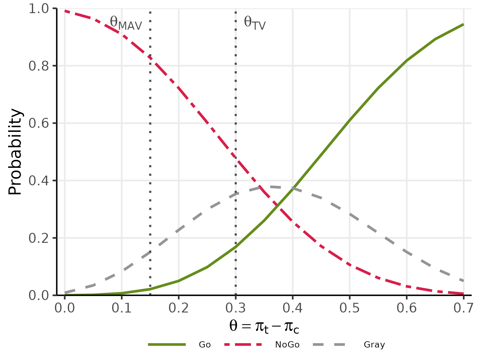

The same function supports design = 'uncontrolled' (with argument z), design = 'external' (with power prior arguments ne_t, ne_c, ye_t, ye_c, alpha0e_t, alpha0e_c), and prob = 'predictive' (with future sample size arguments m_t, m_c and theta_NULL). The function signature and output format are identical across all combinations.

5. Optimal Threshold Search

5.1 Objective and Algorithm

The getgamma1bin() function finds the optimal pair $(\gamma_{\mathrm{go}}^*, \gamma_{\mathrm{nogo}}^*)$ by grid search over $\Gamma = \{\gamma^{(1)}, \ldots, \gamma^{(K)}\} \subset (0, 1)$ at a null scenario $(\pi_t^{\mathrm{null}}, \pi_c^{\mathrm{null}})$ .

A two-stage precompute-then-sweep strategy is used:

Stage 1 (Precompute): all posterior/predictive probabilities $g_{\mathrm{Go}}(y_t, y_c)$ and $g_{\mathrm{NoGo}}(y_t, y_c)$ are computed once over all $(n_t + 1)(n_c + 1)$ outcome pairs — independently of $\gamma$ .

Stage 2 (Sweep): for each candidate $\gamma \in \Gamma$ , $\Pr(\mathrm{Go} \mid \gamma)$ and $\Pr(\mathrm{NoGo} \mid \gamma)$ are obtained as weighted sums of indicator functions:

$\Pr(\mathrm{Go} \mid \gamma) = \sum_{y_t, y_c} \mathbf{1}\!\left[g_{\mathrm{Go}}(y_t, y_c) \ge \gamma\right]\, w(y_t, y_c),$

$\Pr(\mathrm{NoGo} \mid \gamma) = \sum_{y_t, y_c} \mathbf{1}\!\left[g_{\mathrm{NoGo}}(y_t, y_c) \ge \gamma\right]\, w(y_t, y_c),$

where $w(y_t, y_c) = \mathrm{Binom}(y_t; n_t, \pi_t)\,\mathrm{Binom}(y_c; n_c, \pi_c)$ are the binomial weights under the null scenario. No further calls to pbayespostpred1bin() are required at this stage.

The sweep is vectorised using outer(), making the full grid search computationally negligible once Stage 1 is complete.

The optimal $\gamma_{\mathrm{go}}^*$ is the smallest value in $\Gamma$ such that $\Pr(\mathrm{Go} \mid \gamma_{\mathrm{go}}^*)$ satisfies the criterion against a target (e.g., $\Pr(\mathrm{Go}) < 0.05$ ). Analogously for $\gamma_{\mathrm{nogo}}^*$ .

5.2 Example: Controlled Design, Posterior Probability

res_gamma <- getgamma1bin(
  prob      = 'posterior',
  design    = 'controlled',
  theta_TV  = 0.30, theta_MAV = 0.15, theta_NULL = NULL,
  pi_t_go   = 0.10, pi_c_go   = 0.10,
  pi_t_nogo = 0.30, pi_c_nogo = 0.10,
  target_go = 0.05, target_nogo = 0.20,
  n_t = 12L, n_c = 12L,
  a_t = 0.5, b_t = 0.5, a_c = 0.5, b_c = 0.5,
  z = NULL, m_t = NULL, m_c = NULL,
  ne_t = NULL, ne_c = NULL, ye_t = NULL, ye_c = NULL,
  alpha0e_t = NULL, alpha0e_c = NULL,
  gamma_grid = seq(0.01, 0.99, by = 0.01)
)
plot(res_gamma, base_size = 20)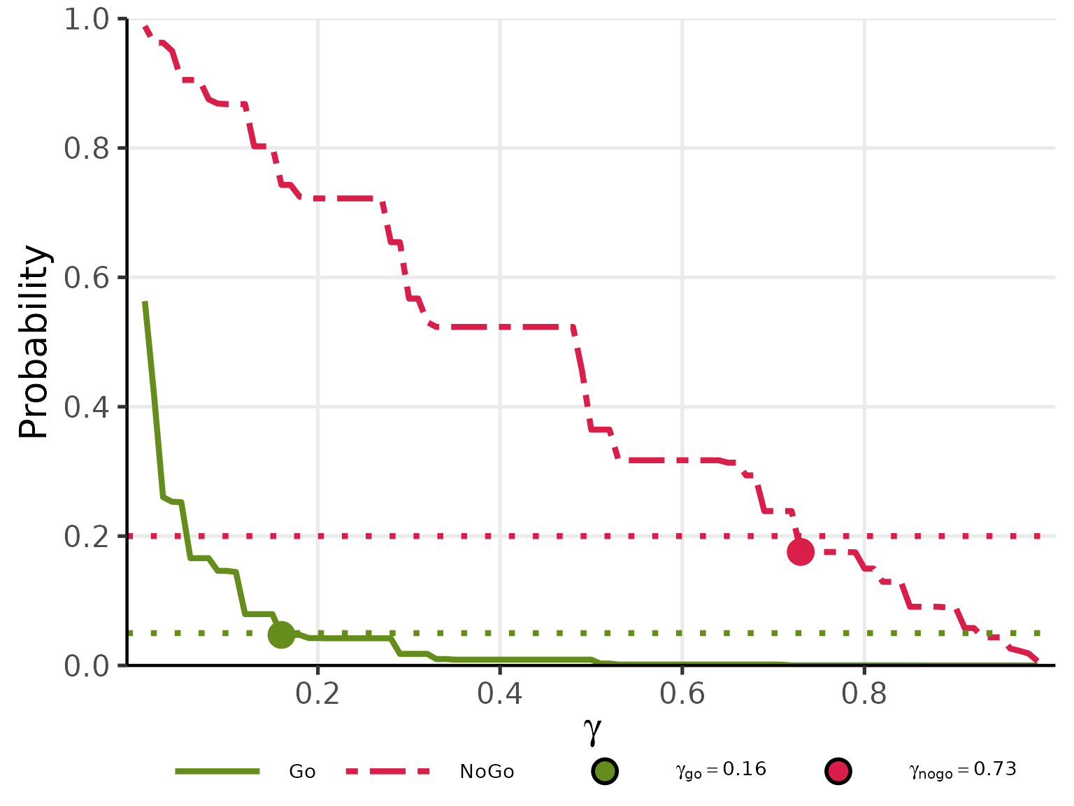

The same function supports design = 'uncontrolled' (with pi_t_go, pi_t_nogo, and z), design = 'external' (with power prior arguments), and prob = 'predictive' (with theta_NULL, m_t, and m_c). The calibration plot and the returned gamma_go/gamma_nogo values are available for all combinations.

6. Summary

This vignette covered single binary endpoint analysis in BayesianQDM:

Bayesian model: Beta-Binomial conjugate posterior with explicit update formulae for $a_j^* = a_j + y_j$ and $b_j^* = b_j + n_j - y_j$ ; Jeffreys prior ( $a_j = b_j = 0.5$ ) as the recommended weakly informative default.
Posterior probability: evaluated via the convolution integral in pbetadiff() — no closed-form CDF exists for the Beta difference.
Posterior predictive probability: evaluated by exact enumeration of the Beta-Binomial double sum in pbetabinomdiff().
Three study designs: controlled (both groups observed), uncontrolled (hypothetical control count $z$ fixed from prior knowledge), external design (power prior with borrowing weight $\alpha_{0ej}$ , augmenting the prior by $\alpha_{0ej}$ times the external sufficient statistics).
Operating characteristics: computed by exact enumeration over all $(n_t+1)(n_c+1)$ outcome pairs with binomial probability weights — no simulation required for the binary endpoint.
Optimal threshold search: two-stage precompute-then-sweep strategy in getgamma1bin() using outer() for a fully vectorised gamma sweep.

See vignette("single-continuous") for the analogous continuous endpoint analysis.