Two Binary Endpoints • BayesianQDM

Motivating Scenario

We extend the single-endpoint RA trial to a bivariate binary design with two co-primary binary endpoints:

Endpoint 1: ACR20 response (1 = responder, 0 = non-responder)
Endpoint 2: DAS28 remission (1 = achieved, 0 = not achieved)

The trial enrolls $n_t = n_c = 7$ patients per group in a 1:1 randomised controlled design.

Clinically meaningful thresholds (posterior probability):

	Endpoint 1	Endpoint 2
$\theta_{\mathrm{TV}1}$	0.20	0.20
$\theta_{\mathrm{MAV}1}$	0.10	0.10

Null hypothesis thresholds (predictive probability): $\theta_{\mathrm{NULL}1} = 0.15$ , $\theta_{\mathrm{NULL}2} = 0.15$ .

Decision thresholds: $\gamma_{\mathrm{go}} = 0.80$ (Go), $\gamma_{\mathrm{nogo}} = 0.80$ (NoGo).

Observed data (used in Sections 2–4): treatment group counts for the four response patterns $(Y_{i,1}, Y_{i,2}) \in \{(0,0),(0,1),(1,0),(1,1)\}$ :

Pattern	Treatment ( $x_{t,lm}$ )	Control ( $x_{c,lm}$ )
(0, 0)	1	2
(0, 1)	1	1
(1, 0)	2	2
(1, 1)	3	2

Marginal responder counts: treatment $y_{t,1} = 5$ , $y_{t,2} = 4$ ; control $y_{c,1} = 4$ , $y_{c,2} = 3$ .

1. Bayesian Model: Dirichlet-Multinomial Conjugate

1.1 Response Pattern Parameterisation

Because the two endpoints within each patient $i$ ( $i = 1, \ldots, n_j$ ) are correlated, the bivariate binary outcome $(Y_{i,1}, Y_{i,2})$ is modelled jointly through its four-cell probability vector

$\mathbf{p}_j = (p_{j,00},\, p_{j,01},\, p_{j,10},\, p_{j,11})^\top, \qquad \mathbf{p}_j \in \Delta^3,$

where $j \in \{t, c\}$ denotes the treatment or control group, $\Delta^3$ denotes the 3-simplex (all entries non-negative and summing to 1), and the subscripts refer to the values of $(Y_{i,1}, Y_{i,2})$ .

The observed count vector $\mathbf{x}_j = (x_{j,00}, x_{j,01}, x_{j,10}, x_{j,11})^\top$ with $\sum_{lm} x_{j,lm} = n_j$ follows

$\mathbf{x}_j \mid \mathbf{p}_j \;\sim\; \mathrm{Multinomial}(n_j,\, \mathbf{p}_j).$

The marginal response rates and treatment effects are obtained by summing:

$\pi_{j1} = p_{j,10} + p_{j,11}, \qquad \pi_{j2} = p_{j,01} + p_{j,11},$

$\theta_1 = \pi_{t1} - \pi_{c1}, \qquad \theta_2 = \pi_{t2} - \pi_{c2}.$

1.2 Prior: Dirichlet Distribution

The conjugate prior for $\mathbf{p}_j$ is the Dirichlet distribution:

$\mathbf{p}_j \;\sim\; \mathrm{Dir}(\alpha_{j,00},\, \alpha_{j,01},\, \alpha_{j,10},\, \alpha_{j,11}),$

where all hyperparameters $\alpha_{j,lm} > 0$ (corresponding to a_t_00, a_t_01, a_t_10, a_t_11 for $j = t$ and a_c_00, a_c_01, a_c_10, a_c_11 for $j = c$ ). The symmetric choice $\alpha_{j,lm} = 0.25$ for all $lm$ is the natural extension of the Jeffreys prior to the four-cell multinomial and is used throughout this vignette.

1.3 Posterior Distribution

By conjugacy of the Dirichlet-Multinomial model, the posterior is:

$\mathbf{p}_j \mid \mathbf{x}_j \;\sim\; \mathrm{Dir}(\alpha_{j,00}^*,\, \alpha_{j,01}^*,\, \alpha_{j,10}^*,\, \alpha_{j,11}^*),$

where the posterior parameters are

$\alpha_{j,lm}^* = \alpha_{j,lm} + x_{j,lm}, \qquad lm \in \{00, 01, 10, 11\}.$

The posterior mean for each cell is $E[p_{j,lm} \mid \mathbf{x}_j] = \alpha_{j,lm}^* / A_j^*$ , where $A_j^* = \sum_{lm} \alpha_{j,lm}^*$ .

1.4 Within-Group Correlation

The within-group Pearson correlation between Endpoint 1 and Endpoint 2 is

$\rho_j = \frac{p_{j,11} - \pi_{j1}\,\pi_{j2}} {\sqrt{\pi_{j1}(1-\pi_{j1})\,\pi_{j2}(1-\pi_{j2})}}.$

When specifying operating characteristic scenarios, the true parameter vector $\mathbf{p}_j$ is specified via the reparameterisation $(\pi_{j1}, \pi_{j2}, \rho_j)$ , with the feasibility constraint:

$\rho_{\min} = \frac{\max(0,\pi_{j1}+\pi_{j2}-1) - \pi_{j1}\pi_{j2}} {\sqrt{\pi_{j1}(1-\pi_{j1})\pi_{j2}(1-\pi_{j2})}} \;\le\; \rho_j \;\le\; \frac{\min(\pi_{j1},\pi_{j2}) - \pi_{j1}\pi_{j2}} {\sqrt{\pi_{j1}(1-\pi_{j1})\pi_{j2}(1-\pi_{j2})}} = \rho_{\max}.$

The helper function getjointbin() converts $(\pi_{j1}, \pi_{j2}, \rho_j)$ to $(p_{j,00}, p_{j,01}, p_{j,10}, p_{j,11})$ :

# Convert marginal rates + correlation to cell probabilities
getjointbin(pi1 = 0.30, pi2 = 0.35, rho = 0.20)
#>      p00      p01      p10      p11 
#> 0.498715 0.201285 0.151285 0.148715
getjointbin(pi1 = 0.20, pi2 = 0.20, rho = 0.00)   # independence
#>  p00  p01  p10  p11 
#> 0.64 0.16 0.16 0.04

1.5 Nine-Region Grid (Posterior Probability)

The bivariate threshold grid for $(\theta_1, \theta_2)$ creates a $3 \times 3$ partition:

Nine-region grid for two-endpoint posterior probability
		Endpoint 1
		θ₁ > θ_TV1	θ_TV1 ≥ θ₁ > θ_MAV1	θ_MAV1 ≥ θ₁
Endpoint 2	θ₂ > θ_TV2	R1	R4	R7
	θ_TV2 ≥ θ₂ > θ_MAV2	R2	R5	R8
	θ_MAV2 ≥ θ₂	R3	R6	R9

Typical choices: Go if $P(R_1) \ge \gamma_{\mathrm{go}}$ , NoGo if $P(R_9) \ge \gamma_{\mathrm{nogo}}$ .

1.6 Four-Region Grid (Predictive Probability)

For the predictive probability, a $2 \times 2$ partition is used:

Four-region grid for two-endpoint predictive probability
		Endpoint 1
		θ₁ > θ_NULL1	θ₁ ≤ θ_NULL1
Endpoint 2	θ₂ > θ_NULL2	R1	R3
Endpoint 2	θ₂ ≤ θ_NULL2	R2	R4

2. Posterior Predictive Distribution

2.1 Dirichlet-Multinomial Predictive Distribution

Let $\tilde{\mathbf{x}}_j \sim \mathrm{Multinomial}(m_j, \mathbf{p}_j)$ be the future count vector with $m_j$ future patients (corresponding to m_t and m_c). Integrating out $\mathbf{p}_j$ over its Dirichlet posterior gives the Dirichlet-Multinomial predictive distribution:

$P(\tilde{\mathbf{x}}_j = \mathbf{c} \mid \mathbf{x}_j) = \binom{m_j}{\mathbf{c}} \frac{B(\boldsymbol{\alpha}_j^* + \mathbf{c})}{B(\boldsymbol{\alpha}_j^*)}, \quad \sum_{lm} c_{lm} = m_j,$

where $B(\cdot)$ is the multivariate Beta function and $\binom{m_j}{\mathbf{c}} = m_j! / \prod_{lm} c_{lm}!$ is the multinomial coefficient.

2.2 Monte Carlo Evaluation

Because the Dirichlet-Multinomial does not yield a tractable closed form for the joint probability that $(\tilde\theta_1, \tilde\theta_2)$ falls in a given region, all region probabilities are estimated by Monte Carlo:

$\widehat{P}(R_r) = \frac{1}{n_\mathrm{MC}} \sum_{s=1}^{n_\mathrm{MC}} \mathbf{1}\!\left[(\pi_{t1}^{(s)} - \pi_{c1}^{(s)},\; \pi_{t2}^{(s)} - \pi_{c2}^{(s)}) \in R_r\right],$

where $\mathbf{p}_j^{(s)} \sim \mathrm{Dir}(\boldsymbol{\alpha}_j^*)$ are draws from the Dirichlet posterior and $\pi_{j1}^{(s)} = p_{j,10}^{(s)} + p_{j,11}^{(s)}$ , $\pi_{j2}^{(s)} = p_{j,01}^{(s)} + p_{j,11}^{(s)}$ . For the predictive probability, future proportion differences $\tilde\theta_k^{(s)} = \tilde{\pi}_{t,k}^{(s)} - \tilde{\pi}_{c,k}^{(s)}$ are computed from corresponding Multinomial draws conditioned on the Dirichlet samples.

3. Study Designs

3.1 Controlled Design

Both groups are observed in the PoC trial. The posterior parameters are updated as $\alpha_{j,lm}^* = \alpha_{j,lm} + x_{j,lm}$ , where $(x_{t,00}, x_{t,01}, x_{t,10}, x_{t,11})$ and $(x_{c,00}, x_{c,01}, x_{c,10}, x_{c,11})$ are supplied as x_t_00, …, x_t_11 and x_c_00, …, x_c_11.

set.seed(42)
p_post_ctrl <- pbayespostpred2bin(
  prob = 'posterior', design = 'controlled',
  theta_TV1 = 0.20, theta_MAV1 = 0.10,
  theta_TV2 = 0.20, theta_MAV2 = 0.10,
  theta_NULL1 = NULL, theta_NULL2 = NULL,
  x_t_00 = 1L, x_t_01 = 1L, x_t_10 = 2L, x_t_11 = 3L,
  x_c_00 = 2L, x_c_01 = 1L, x_c_10 = 2L, x_c_11 = 2L,
  a_t_00 = 0.25, a_t_01 = 0.25, a_t_10 = 0.25, a_t_11 = 0.25,
  a_c_00 = 0.25, a_c_01 = 0.25, a_c_10 = 0.25, a_c_11 = 0.25,
  m_t = NULL, m_c = NULL,
  z00 = NULL, z01 = NULL, z10 = NULL, z11 = NULL,
  xe_t_00 = NULL, xe_t_01 = NULL, xe_t_10 = NULL, xe_t_11 = NULL,
  xe_c_00 = NULL, xe_c_01 = NULL, xe_c_10 = NULL, xe_c_11 = NULL,
  alpha0e_t = NULL, alpha0e_c = NULL,
  nMC = 1000L
)
print(round(p_post_ctrl, 4))
#>    R1    R2    R3    R4    R5    R6    R7    R8    R9 
#> 0.174 0.075 0.133 0.075 0.025 0.083 0.149 0.069 0.217
cat(sprintf(
  "\nGo  region (R1): P = %.4f  >= gamma_go (0.80)? %s\n",
  p_post_ctrl["R1"], ifelse(p_post_ctrl["R1"] >= 0.80, "YES -> Go", "NO")
))
#> 
#> Go  region (R1): P = 0.1740  >= gamma_go (0.80)? NO
cat(sprintf(
  "NoGo region (R9): P = %.4f  >= gamma_nogo (0.80)? %s\n",
  p_post_ctrl["R9"], ifelse(p_post_ctrl["R9"] >= 0.80, "YES -> NoGo", "NO")
))
#> NoGo region (R9): P = 0.2170  >= gamma_nogo (0.80)? NO

Posterior predictive probability (future Phase III: $m_t = m_c = 15$ ):

set.seed(42)
p_pred_ctrl <- pbayespostpred2bin(
  prob = 'predictive', design = 'controlled',
  theta_TV1 = NULL, theta_MAV1 = NULL,
  theta_TV2 = NULL, theta_MAV2 = NULL,
  theta_NULL1 = 0.15, theta_NULL2 = 0.15,
  x_t_00 = 1L, x_t_01 = 1L, x_t_10 = 2L, x_t_11 = 3L,
  x_c_00 = 2L, x_c_01 = 1L, x_c_10 = 2L, x_c_11 = 2L,
  a_t_00 = 0.25, a_t_01 = 0.25, a_t_10 = 0.25, a_t_11 = 0.25,
  a_c_00 = 0.25, a_c_01 = 0.25, a_c_10 = 0.25, a_c_11 = 0.25,
  m_t = 15L, m_c = 15L,
  z00 = NULL, z01 = NULL, z10 = NULL, z11 = NULL,
  xe_t_00 = NULL, xe_t_01 = NULL, xe_t_10 = NULL, xe_t_11 = NULL,
  xe_c_00 = NULL, xe_c_01 = NULL, xe_c_10 = NULL, xe_c_11 = NULL,
  alpha0e_t = NULL, alpha0e_c = NULL,
  nMC = 1000L
)
print(round(p_pred_ctrl, 4))
#>    R1    R2    R3    R4 
#> 0.247 0.221 0.236 0.296
cat(sprintf(
  "\nGo region (R1): P = %.4f  >= gamma_go (0.80)? %s\n",
  p_pred_ctrl["R1"], ifelse(p_pred_ctrl["R1"] >= 0.80, "YES -> Go", "NO")
))
#> 
#> Go region (R1): P = 0.2470  >= gamma_go (0.80)? NO

3.2 Uncontrolled Design

When no concurrent control group is enrolled, the control distribution is specified via a hypothetical count vector $\mathbf{z} = (z_{00}, z_{01}, z_{10}, z_{11})$ combined with the Dirichlet prior:

$\mathbf{p}_c \;\sim\; \mathrm{Dir}(\alpha_{c,00} + z_{00},\; \alpha_{c,01} + z_{01},\; \alpha_{c,10} + z_{10},\; \alpha_{c,11} + z_{11}).$

This specification encodes prior belief about the bivariate control response rates — including any assumed within-group correlation — without requiring observed control data. The hypothetical counts are supplied as z00, z01, z10, z11.

set.seed(1)
p_unctrl <- pbayespostpred2bin(
  prob = 'posterior', design = 'uncontrolled',
  theta_TV1 = 0.20, theta_MAV1 = 0.10,
  theta_TV2 = 0.20, theta_MAV2 = 0.10,
  theta_NULL1 = NULL, theta_NULL2 = NULL,
  x_t_00 = 1L, x_t_01 = 1L, x_t_10 = 2L, x_t_11 = 3L,
  x_c_00 = NULL, x_c_01 = NULL, x_c_10 = NULL, x_c_11 = NULL,
  a_t_00 = 0.25, a_t_01 = 0.25, a_t_10 = 0.25, a_t_11 = 0.25,
  a_c_00 = 0.25, a_c_01 = 0.25, a_c_10 = 0.25, a_c_11 = 0.25,
  m_t = NULL, m_c = NULL,
  z00 = 2L, z01 = 1L, z10 = 2L, z11 = 1L,
  xe_t_00 = NULL, xe_t_01 = NULL, xe_t_10 = NULL, xe_t_11 = NULL,
  xe_c_00 = NULL, xe_c_01 = NULL, xe_c_10 = NULL, xe_c_11 = NULL,
  alpha0e_t = NULL, alpha0e_c = NULL,
  nMC = 1000L
)
print(round(p_unctrl, 4))
#>    R1    R2    R3    R4    R5    R6    R7    R8    R9 
#> 0.262 0.075 0.142 0.083 0.026 0.058 0.193 0.056 0.105

3.3 External Control Design (Power Prior)

External data for group $j$ (count vector $\mathbf{x}_{ej}$ , supplied as xe_t_00, …, xe_t_11 for $j = t$ and xe_c_00, …, xe_c_11 for $j = c$ ) are incorporated via a Dirichlet power prior with weight $\alpha_{0e,j} \in (0, 1]$ (alpha0e_t, alpha0e_c). The augmented prior parameters are:

$\alpha_{j,lm}^{*} = \alpha_{j,lm} + \alpha_{0e,j} \cdot x_{ej,lm}.$

Setting $\alpha_{0e,j} = 1$ treats the external data as equivalent to current trial data; $\alpha_{0e,j} \to 0$ recovers the original prior. The current PoC data then update these augmented parameters:

$\alpha_{j,lm}^{**} = \alpha_{j,lm}^{*} + x_{j,lm} = \alpha_{j,lm} + \alpha_{0e,j}\, x_{ej,lm} + x_{j,lm}.$

When only the control group uses external data (external control design), xe_t_00 through xe_t_11 and alpha0e_t are set to NULL.

set.seed(2)
p_ext <- pbayespostpred2bin(
  prob = 'posterior', design = 'external',
  theta_TV1 = 0.20, theta_MAV1 = 0.10,
  theta_TV2 = 0.20, theta_MAV2 = 0.10,
  theta_NULL1 = NULL, theta_NULL2 = NULL,
  x_t_00 = 1L, x_t_01 = 1L, x_t_10 = 2L, x_t_11 = 3L,
  x_c_00 = 2L, x_c_01 = 1L, x_c_10 = 2L, x_c_11 = 2L,
  a_t_00 = 0.25, a_t_01 = 0.25, a_t_10 = 0.25, a_t_11 = 0.25,
  a_c_00 = 0.25, a_c_01 = 0.25, a_c_10 = 0.25, a_c_11 = 0.25,
  m_t = NULL, m_c = NULL,
  z00 = NULL, z01 = NULL, z10 = NULL, z11 = NULL,
  xe_t_00 = NULL, xe_t_01 = NULL, xe_t_10 = NULL, xe_t_11 = NULL,
  xe_c_00 = 3L,   xe_c_01 = 1L,   xe_c_10 = 2L,   xe_c_11 = 1L,
  alpha0e_t = NULL, alpha0e_c = 0.5,
  nMC = 1000L
)
print(round(p_ext, 4))
#>    R1    R2    R3    R4    R5    R6    R7    R8    R9 
#> 0.215 0.072 0.151 0.087 0.036 0.078 0.151 0.075 0.135

Sensitivity to borrowing weight $\alpha_{0e,c}$ :

ae_seq <- c(0.01, seq(0.1, 1.0, by = 0.1))
p_ae <- sapply(ae_seq, function(ae) {
  set.seed(99)
  res <- pbayespostpred2bin(
    prob = 'posterior', design = 'external',
    theta_TV1 = 0.20, theta_MAV1 = 0.10,
    theta_TV2 = 0.20, theta_MAV2 = 0.10,
    theta_NULL1 = NULL, theta_NULL2 = NULL,
    x_t_00 = 1L, x_t_01 = 1L, x_t_10 = 2L, x_t_11 = 3L,
    x_c_00 = 2L, x_c_01 = 1L, x_c_10 = 2L, x_c_11 = 2L,
    a_t_00 = 0.25, a_t_01 = 0.25, a_t_10 = 0.25, a_t_11 = 0.25,
    a_c_00 = 0.25, a_c_01 = 0.25, a_c_10 = 0.25, a_c_11 = 0.25,
    m_t = NULL, m_c = NULL,
    z00 = NULL, z01 = NULL, z10 = NULL, z11 = NULL,
    xe_t_00 = NULL, xe_t_01 = NULL, xe_t_10 = NULL, xe_t_11 = NULL,
    xe_c_00 = 3L,   xe_c_01 = 1L,   xe_c_10 = 2L,   xe_c_11 = 1L,
    alpha0e_t = NULL, alpha0e_c = ae, nMC = 500L
  )
  res["R1"]
})
data.frame(alpha0e_c = ae_seq, P_R1 = round(p_ae, 4))
#>    alpha0e_c  P_R1
#> 1       0.01 0.142
#> 2       0.10 0.164
#> 3       0.20 0.184
#> 4       0.30 0.180
#> 5       0.40 0.196
#> 6       0.50 0.208
#> 7       0.60 0.220
#> 8       0.70 0.246
#> 9       0.80 0.230
#> 10      0.90 0.228
#> 11      1.00 0.238

4. Operating Characteristics

4.1 Definition

For given true parameters $(\mathbf{p}_t, \mathbf{p}_c)$ , the operating characteristics are computed by exact enumeration over all possible multinomial count combinations via a two-stage strategy.

Stage 1 (precomputation): all count combinations $\mathbf{x}_{t,i}$ ( $K_t$ combinations) and $\mathbf{x}_{c,j}$ ( $K_c$ combinations) are enumerated by allmultinom(). For each pair $(i, j)$ , pbayespostpred2bin() computes the region probability vector once, yielding $\hat{g}_{\mathrm{go},ij}$ and $\hat{g}_{\mathrm{nogo},ij}$ independent of any decision threshold.

Stage 2 (weighting): for given thresholds $(\gamma_{\mathrm{go}}, \gamma_{\mathrm{nogo}})$ :

$\Pr(\mathrm{Go}) = \sum_{i=1}^{K_t} \sum_{j=1}^{K_c} w_{ij}\, \mathbf{1}\!\left[\hat{g}_{\mathrm{go},ij} \ge \gamma_{\mathrm{go}} \text{ and } \hat{g}_{\mathrm{nogo},ij} < \gamma_{\mathrm{nogo}}\right],$

$\Pr(\mathrm{NoGo}) = \sum_{i=1}^{K_t} \sum_{j=1}^{K_c} w_{ij}\, \mathbf{1}\!\left[\hat{g}_{\mathrm{nogo},ij} \ge \gamma_{\mathrm{nogo}} \text{ and } \hat{g}_{\mathrm{go},ij} < \gamma_{\mathrm{go}}\right],$

where $w_{ij} = P_\mathrm{Mult}(\mathbf{x}_{t,i};\, n_t, \mathbf{p}_t) \times P_\mathrm{Mult}(\mathbf{x}_{c,j};\, n_c, \mathbf{p}_c)$ , and

$\hat{g}_{\mathrm{go},ij} = \sum_{r \in \text{GoRegions}} \hat{P}(R_r \mid \mathbf{x}_{t,i}, \mathbf{x}_{c,j}),$ $\hat{g}_{\mathrm{nogo},ij} = \sum_{r \in \text{NoGoRegions}} \hat{P}(R_r \mid \mathbf{x}_{t,i}, \mathbf{x}_{c,j}).$

A Miss ( $\hat{g}_{\mathrm{go},ij} \ge \gamma_{\mathrm{go}}$ AND $\hat{g}_{\mathrm{nogo},ij} \ge \gamma_{\mathrm{nogo}}$ ) indicates an inconsistent threshold configuration and triggers an error by default (error_if_Miss = TRUE). Gray comprises all remaining outcomes.

For large $n_t$ or $n_c$ , the CalcMethod = 'MC' option replaces full enumeration with $n_\mathrm{sim}$ multinomial draws, deduplicates them into $K \ll n_\mathrm{sim}$ unique pairs, and evaluates pbayespostpred2bin() only for those unique pairs.

Note on computation time. The number of multinomial count combinations grows rapidly with $n$ : for $n_j$ patients and 4 response categories the number of combinations is $\binom{n_j + 3}{3}$ , which equals 286 for $n_j = 10$ and 1771 for $n_j = 20$ . For the Exact method with two groups this means up to $286^2 \approx 82{,}000$ unique pairs each requiring nMC Dirichlet draws. When predictive probability is used ( $m_j > 0$ ), an additional layer of Multinomial sampling is added inside each Dirichlet draw, further multiplying computation time. Use small nMC (100–500) and n_t = n_c = 10 for demonstration; switch to CalcMethod = 'MC' with moderate nsim for larger sample sizes.

4.2 Example: Controlled Design, Posterior Probability

pi_t_seq <- seq(0.20, 0.90, by = 0.10)
n_scen   <- length(pi_t_seq)

oc_ctrl <- pbayesdecisionprob2bin(
  prob = 'posterior', design = 'controlled',
  GoRegions = 1L, NoGoRegions = 9L,
  gamma_go = 0.80, gamma_nogo = 0.80,
  pi_t1 = rep(pi_t_seq, each = n_scen),
  pi_t2 = rep(pi_t_seq, times = n_scen),
  rho_t = rep(0.0, n_scen * n_scen),
  pi_c1 = rep(0.20, n_scen * n_scen),
  pi_c2 = rep(0.20, n_scen * n_scen),
  rho_c = rep(0.0,  n_scen * n_scen),
  n_t = 7L, n_c = 7L,
  a_t_00 = 0.25, a_t_01 = 0.25, a_t_10 = 0.25, a_t_11 = 0.25,
  a_c_00 = 0.25, a_c_01 = 0.25, a_c_10 = 0.25, a_c_11 = 0.25,
  m_t = NULL, m_c = NULL,
  theta_TV1  = 0.20, theta_MAV1 = 0.10,
  theta_TV2  = 0.20, theta_MAV2 = 0.10,
  theta_NULL1 = NULL, theta_NULL2 = NULL,
  z00 = NULL, z01 = NULL, z10 = NULL, z11 = NULL,
  xe_t_00 = NULL, xe_t_01 = NULL, xe_t_10 = NULL, xe_t_11 = NULL,
  xe_c_00 = NULL, xe_c_01 = NULL, xe_c_10 = NULL, xe_c_11 = NULL,
  alpha0e_t = NULL, alpha0e_c = NULL,
  nMC = 200L, CalcMethod = 'Exact',
  error_if_Miss = TRUE, Gray_inc_Miss = FALSE
)
print(oc_ctrl)
#> Go/NoGo/Gray Decision Probabilities (Two Binary Endpoints) 
#> ----------------------------------------------------------------------------- 
#>   Probability type : posterior 
#>   Design           : controlled 
#>   Threshold(s)     : TV1 = 0.2, MAV1 = 0.1 
#>                      TV2 = 0.2, MAV2 = 0.1 
#>   Go  threshold    : gamma_go = 0.8 
#>   NoGo threshold   : gamma_nogo = 0.8 
#>   Go  regions      : {1} 
#>   NoGo regions     : {9} 
#>   Sample size      : n_t = 7, n_c = 7 
#>   Prior (treatment): a_t = (0.25, 0.25, 0.25, 0.25)  [a_00, a_01, a_10, a_11] 
#>   Prior (control)  : a_c = (0.25, 0.25, 0.25, 0.25)  [a_00, a_01, a_10, a_11] 
#>   Method           : Exact 
#>   MC draws         : nMC = 200 
#>   Miss handling    : error_if_Miss = TRUE, Gray_inc_Miss = FALSE 
#> ----------------------------------------------------------------------------- 
#>  pi_t1 pi_t2 rho_t pi_c1 pi_c2 rho_c     Go   Gray   NoGo
#>    0.2   0.2     0   0.2   0.2     0 0.0002 0.8886 0.1112
#>    0.2   0.3     0   0.2   0.2     0 0.0008 0.9381 0.0611
#>    0.2   0.4     0   0.2   0.2     0 0.0021 0.9666 0.0313
#>    0.2   0.5     0   0.2   0.2     0 0.0045 0.9810 0.0145
#>    0.2   0.6     0   0.2   0.2     0 0.0082 0.9859 0.0059
#>    0.2   0.7     0   0.2   0.2     0 0.0136 0.9845 0.0019
#>    0.2   0.8     0   0.2   0.2     0 0.0205 0.9791 0.0004
#>    0.2   0.9     0   0.2   0.2     0 0.0290 0.9710 0.0000
#>    0.3   0.2     0   0.2   0.2     0 0.0009 0.9380 0.0611
#>    0.3   0.3     0   0.2   0.2     0 0.0031 0.9637 0.0332
#>    0.3   0.4     0   0.2   0.2     0 0.0076 0.9756 0.0168
#>    0.3   0.5     0   0.2   0.2     0 0.0151 0.9772 0.0077
#>    0.3   0.6     0   0.2   0.2     0 0.0262 0.9707 0.0030
#>    0.3   0.7     0   0.2   0.2     0 0.0415 0.9575 0.0010
#>    0.3   0.8     0   0.2   0.2     0 0.0610 0.9388 0.0002
#>    0.3   0.9     0   0.2   0.2     0 0.0848 0.9152 0.0000
#>    0.4   0.2     0   0.2   0.2     0 0.0024 0.9670 0.0306
#>    0.4   0.3     0   0.2   0.2     0 0.0080 0.9755 0.0165
#>    0.4   0.4     0   0.2   0.2     0 0.0186 0.9732 0.0082
#>    0.4   0.5     0   0.2   0.2     0 0.0352 0.9611 0.0037
#>    0.4   0.6     0   0.2   0.2     0 0.0586 0.9400 0.0014
#>    0.4   0.7     0   0.2   0.2     0 0.0892 0.9104 0.0005
#>    0.4   0.8     0   0.2   0.2     0 0.1272 0.8728 0.0000
#>    0.4   0.9     0   0.2   0.2     0 0.1728 0.8272 0.0000
#>    0.5   0.2     0   0.2   0.2     0 0.0053 0.9811 0.0136
#>    0.5   0.3     0   0.2   0.2     0 0.0167 0.9761 0.0073
#>    0.5   0.4     0   0.2   0.2     0 0.0368 0.9596 0.0036
#>    0.5   0.5     0   0.2   0.2     0 0.0667 0.9317 0.0016
#>    0.5   0.6     0   0.2   0.2     0 0.1070 0.8924 0.0006
#>    0.5   0.7     0   0.2   0.2     0 0.1574 0.8424 0.0002
#>    0.5   0.8     0   0.2   0.2     0 0.2176 0.7824 0.0000
#>    0.5   0.9     0   0.2   0.2     0 0.2876 0.7124 0.0000
#>    0.6   0.2     0   0.2   0.2     0 0.0098 0.9850 0.0051
#>    0.6   0.3     0   0.2   0.2     0 0.0296 0.9677 0.0027
#>    0.6   0.4     0   0.2   0.2     0 0.0628 0.9359 0.0013
#>    0.6   0.5     0   0.2   0.2     0 0.1101 0.8894 0.0006
#>    0.6   0.6     0   0.2   0.2     0 0.1709 0.8289 0.0002
#>    0.6   0.7     0   0.2   0.2     0 0.2440 0.7560 0.0000
#>    0.6   0.8     0   0.2   0.2     0 0.3274 0.6726 0.0000
#>    0.6   0.9     0   0.2   0.2     0 0.4198 0.5802 0.0000
#>    0.7   0.2     0   0.2   0.2     0 0.0161 0.9824 0.0016
#>    0.7   0.3     0   0.2   0.2     0 0.0466 0.9526 0.0008
#>    0.7   0.4     0   0.2   0.2     0 0.0958 0.9038 0.0004
#>    0.7   0.5     0   0.2   0.2     0 0.1632 0.8366 0.0002
#>    0.7   0.6     0   0.2   0.2     0 0.2470 0.7530 0.0000
#>    0.7   0.7     0   0.2   0.2     0 0.3437 0.6563 0.0000
#>    0.7   0.8     0   0.2   0.2     0 0.4488 0.5512 0.0000
#>    0.7   0.9     0   0.2   0.2     0 0.5577 0.4423 0.0000
#>    0.8   0.2     0   0.2   0.2     0 0.0235 0.9762 0.0003
#>    0.8   0.3     0   0.2   0.2     0 0.0663 0.9335 0.0002
#>    0.8   0.4     0   0.2   0.2     0 0.1331 0.8669 0.0000
#>    0.8   0.5     0   0.2   0.2     0 0.2221 0.7779 0.0000
#>    0.8   0.6     0   0.2   0.2     0 0.3295 0.6705 0.0000
#>    0.8   0.7     0   0.2   0.2     0 0.4491 0.5509 0.0000
#>    0.8   0.8     0   0.2   0.2     0 0.5724 0.4276 0.0000
#>    0.8   0.9     0   0.2   0.2     0 0.6897 0.3103 0.0000
#>    0.9   0.2     0   0.2   0.2     0 0.0310 0.9690 0.0000
#>    0.9   0.3     0   0.2   0.2     0 0.0861 0.9139 0.0000
#>    0.9   0.4     0   0.2   0.2     0 0.1702 0.8298 0.0000
#>    0.9   0.5     0   0.2   0.2     0 0.2804 0.7196 0.0000
#>    0.9   0.6     0   0.2   0.2     0 0.4108 0.5892 0.0000
#>    0.9   0.7     0   0.2   0.2     0 0.5518 0.4482 0.0000
#>    0.9   0.8     0   0.2   0.2     0 0.6892 0.3108 0.0000
#>    0.9   0.9     0   0.2   0.2     0 0.8073 0.1927 0.0000
#> -----------------------------------------------------------------------------
plot(oc_ctrl, base_size = 20)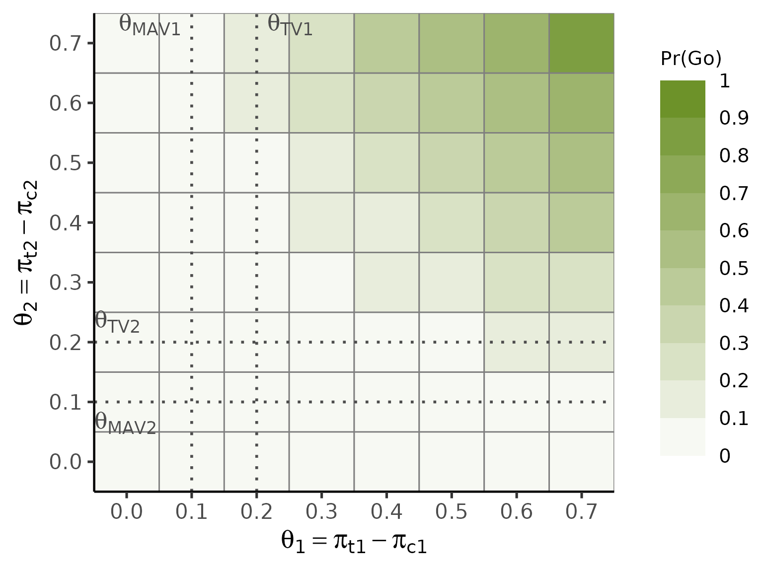

The same function supports design = 'uncontrolled' (with hypothetical count vector arguments z00, z01, z10, z11), design = 'external' (with power prior arguments xe_c_00, …, xe_c_11 and alpha0e_c), and prob = 'predictive' (with future sample size arguments m_t, m_c and theta_NULL1, theta_NULL2). The within-group correlation rho_t can also be varied to study its effect on the operating characteristics. The function signature and output format are identical across all combinations.

5. Optimal Threshold Search

5.1 Objective and Algorithm

getgamma2bin() finds the optimal pair $(\gamma_{\mathrm{go}}^*, \gamma_{\mathrm{nogo}}^*)$ by the same two-stage precompute-then-sweep strategy as pbayesdecisionprob2bin(), but sweeps over the two-dimensional grid $\Gamma_{\mathrm{go}} \times \Gamma_{\mathrm{nogo}}$ (gamma_go_grid $\times$ gamma_nogo_grid). The two thresholds are calibrated independently under separate scenarios:

$\gamma_{\mathrm{go}}^*$ : calibrated under the Go-calibration scenario (pi_t1_go, pi_t2_go, rho_t_go, pi_c1_go, pi_c2_go, rho_c_go; typically the null scenario $\pi_t = \pi_c$ ), so that $\Pr(\mathrm{Go}) < \texttt{target_go}$ .
$\gamma_{\mathrm{nogo}}^*$ : calibrated under the NoGo-calibration scenario (pi_t1_nogo, pi_t2_nogo, rho_t_nogo, pi_c1_nogo, pi_c2_nogo, rho_c_nogo; typically the alternative scenario), so that $\Pr(\mathrm{NoGo}) < \texttt{target_nogo}$ .

Stage 1 (precomputation): pbayespostpred2bin() is called for every unique multinomial outcome combination $(\mathbf{x}_{t,i}, \mathbf{x}_{c,j})$ enumerated by allmultinom(). The region probability vector is summed over GoRegions and NoGoRegions to obtain $\hat{g}_{\mathrm{go},ij}$ and $\hat{g}_{\mathrm{nogo},ij}$ , independent of $(\gamma_{\mathrm{go}}, \gamma_{\mathrm{nogo}})$ .

Stage 2 (gamma sweep): for every pair $(\gamma_{\mathrm{go}}, \gamma_{\mathrm{nogo}}) \in \Gamma_{\mathrm{go}} \times \Gamma_{\mathrm{nogo}}$ :

$\Pr(\mathrm{Go} \mid \gamma_{\mathrm{go}}, \gamma_{\mathrm{nogo}}) = \sum_{i,j} w_{ij}\, \mathbf{1}\!\left[\hat{g}_{\mathrm{go},ij} \ge \gamma_{\mathrm{go}} \text{ and } \hat{g}_{\mathrm{nogo},ij} < \gamma_{\mathrm{nogo}}\right],$

$\Pr(\mathrm{NoGo} \mid \gamma_{\mathrm{go}}, \gamma_{\mathrm{nogo}}) = \sum_{i,j} w_{ij}\, \mathbf{1}\!\left[\hat{g}_{\mathrm{nogo},ij} \ge \gamma_{\mathrm{nogo}} \text{ and } \hat{g}_{\mathrm{go},ij} < \gamma_{\mathrm{go}}\right].$

Results are stored in $|\Gamma_{\mathrm{go}}| \times |\Gamma_{\mathrm{nogo}}|$ matrices PrGo_grid and PrNoGo_grid.

Stage 3 (optimal selection): for each candidate $\gamma_{\mathrm{go}}$ , the worst-case $\Pr(\mathrm{Go})$ over all $\gamma_{\mathrm{nogo}}$ is compared against target_go; analogously for $\gamma_{\mathrm{nogo}}$ .

5.2 Example: Controlled Design, Posterior Probability

Null scenario: $\pi_{t1} = \pi_{c1} = 0.20$ , $\pi_{t2} = \pi_{c2} = 0.20$ , $\rho_t = \rho_c = 0$ (no treatment effect, independence).

res_gamma <- getgamma2bin(
  prob = 'posterior', design = 'controlled',
  GoRegions = 1L, NoGoRegions = 9L,
  pi_t1_go = 0.20, pi_t2_go = 0.20, rho_t_go = 0.0,
  pi_c1_go = 0.20, pi_c2_go = 0.20, rho_c_go = 0.0,
  pi_t1_nogo = 0.40, pi_t2_nogo = 0.40, rho_t_nogo = 0.0,
  pi_c1_nogo = 0.20, pi_c2_nogo = 0.20, rho_c_nogo = 0.0,
  target_go = 0.05, target_nogo = 0.20,
  n_t = 7L, n_c = 7L,
  a_t_00 = 0.25, a_t_01 = 0.25, a_t_10 = 0.25, a_t_11 = 0.25,
  a_c_00 = 0.25, a_c_01 = 0.25, a_c_10 = 0.25, a_c_11 = 0.25,
  theta_TV1  = 0.20, theta_MAV1 = 0.10,
  theta_TV2  = 0.20, theta_MAV2 = 0.10,
  theta_NULL1 = NULL, theta_NULL2 = NULL,
  m_t = NULL, m_c = NULL,
  z00 = NULL, z01 = NULL, z10 = NULL, z11 = NULL,
  xe_t_00 = NULL, xe_t_01 = NULL, xe_t_10 = NULL, xe_t_11 = NULL,
  xe_c_00 = NULL, xe_c_01 = NULL, xe_c_10 = NULL, xe_c_11 = NULL,
  alpha0e_t = NULL, alpha0e_c = NULL,
  nMC = 200L,
  gamma_go_grid   = seq(0.05, 0.95, by = 0.05),
  gamma_nogo_grid = seq(0.05, 0.95, by = 0.05)
)
plot(res_gamma, base_size = 20)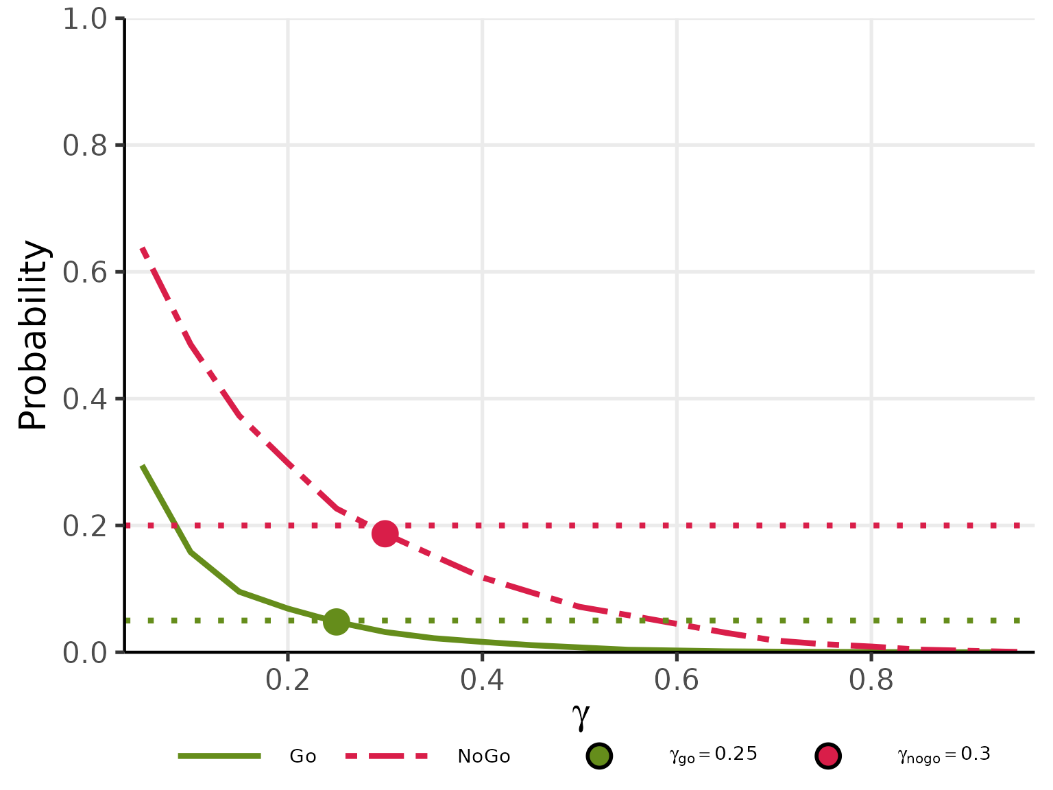

The same function supports design = 'uncontrolled' (with pi_t1_go, pi_t2_go, rho_t_go, pi_t1_nogo, pi_t2_nogo, rho_t_nogo; set pi_c*_go and pi_c*_nogo to NULL), design = 'external' (with power prior arguments), and prob = 'predictive' (with theta_NULL1, theta_NULL2, m_t, and m_c). The calibration plot and the returned gamma_go/gamma_nogo values are available for all combinations.

6. Summary

This vignette covered two binary endpoint analysis in BayesianQDM:

Bayesian model: Dirichlet-Multinomial conjugate, modelling the bivariate binary outcome through the four-cell probability vector $\mathbf{p}_j$ ( $j \in \{t, c\}$ ). Posterior update: $\alpha_{j,lm}^* = \alpha_{j,lm} + x_{j,lm}$ . The symmetric Jeffreys-type prior $\alpha_{j,lm} = 0.25$ is recommended.
Within-group correlation: parameterised via $\rho_j$ using the moment-matching identity; feasible range enforced by getjointbin().
Nine-region grid for posterior probability and four-region grid for predictive probability, identical in structure to the two continuous endpoint case.
Monte Carlo evaluation of region probabilities via Dirichlet draws; no closed-form expression for the joint probability exists in the bivariate binary case.
Three study designs: controlled design (standard posterior update), uncontrolled design (hypothetical count vector $\mathbf{z}$ fixes the control Dirichlet distribution), external control design (Dirichlet power prior with $\alpha_{j,lm}^* = \alpha_{j,lm} + \alpha_{0e,j}\, x_{ej,lm}$ ).
Exact operating characteristics: two-stage precomputation over all multinomial count combinations via allmultinom(), with multinomial probability weighting (no outer Monte Carlo needed for small $n$ ).
Optimal threshold search: three-stage precompute-then-sweep in getgamma2bin(), producing $|\Gamma_{\mathrm{go}}| \times |\Gamma_{\mathrm{nogo}}|$ matrices PrGo_grid and PrNoGo_grid, visualised as contour plots.

See vignette("overview") for a comparison across all four endpoint types.