Two Continuous Endpoints

Motivating Scenario

We extend the single-endpoint RA trial to a bivariate design with two co-primary continuous endpoints:

• Endpoint 1: change from baseline in DAS28 score
• Endpoint 2: change from baseline in HAQ-DI (Health Assessment Questionnaire – Disability Index)

The trial enrolls $n_t = n_c = 20$ patients per group (treatment vs. placebo) in a 1:1 randomised controlled design.

Clinically meaningful thresholds (posterior probability):

	Endpoint 1	Endpoint 2
$\theta_{\mathrm{TV},1}$	1.5	1.0
$\theta_{\mathrm{MAV},1}$	0.5	0.3

Null hypothesis thresholds (predictive probability): $\theta_{\mathrm{NULL},1} = 0.5$, $\theta_{\mathrm{NULL},2} = 0.3$.

Decision thresholds: $\gamma_1 = 0.80$ (Go), $\gamma_2 = 0.20$ (NoGo).

Observed data (used in Sections 2–4):

• Treatment: $\bar{\mathbf{y}}_t = (3.5, 2.1)^\top$, $S_t = \begin{pmatrix}18.0 & 3.6\\3.6 & 9.0\end{pmatrix}$
• Control: $\bar{\mathbf{y}}_c = (1.8, 1.0)^\top$, $S_c = \begin{pmatrix}16.0 & 2.8\\2.8 & 8.5\end{pmatrix}$

where $S_j = \sum_{i=1}^{n_j}(\mathbf{y}_{ij} - \bar{\mathbf{y}}_j) (\mathbf{y}_{ij} - \bar{\mathbf{y}}_j)^\top$ ($j = t, c$) is the sum-of-squares matrix.

---

1. Bayesian Model: Normal-Inverse-Wishart Conjugate

1.1 Prior Distribution

For group $j$ ($j = t$: treatment, $j = c$: control), we model the bivariate outcomes for patient $i$ ($i = 1, \ldots, n_j$) as

$$\mathbf{y}_{ij} \mid \boldsymbol{\mu}_j, \Sigma_j \;\overset{iid}{\sim}\; \mathcal{N}_2(\boldsymbol{\mu}_j,\, \Sigma_j).$$

The conjugate prior is the Normal-Inverse-Wishart (NIW) distribution:

$$(\boldsymbol{\mu}_j, \Sigma_j) \;\sim\; \mathrm{NIW}(\boldsymbol{\mu}_{0j},\, \kappa_{0j},\, \nu_{0j},\, \Lambda_{0j}),$$

where $\boldsymbol{\mu}_{0j} \in \mathbb{R}^2$ is the prior mean (argument mu0_t or mu0_c), $\kappa_{0j} > 0$ is the prior concentration (kappa0_t or kappa0_c), $\nu_{0j} > 3$ is the prior degrees of freedom (nu0_t or nu0_c), and $\Lambda_{0j}$ is a $2 \times 2$ positive-definite prior scale matrix (Lambda0_t or Lambda0_c).

The vague (Jeffreys) prior is obtained by letting $\kappa_{0j} \to 0$ and $\nu_{0j} \to 0$ (prior = 'vague').

1.2 Posterior Distribution

Given $n_j$ observations with sample mean $\bar{\mathbf{y}}_j$ (ybar_t or ybar_c) and sum-of-squares matrix $S_j$ (S_t or S_c), the NIW posterior has updated parameters:

$$\kappa_{nj} = \kappa_{0j} + n_j, \qquad \nu_{nj} = \nu_{0j} + n_j,$$

$$\boldsymbol{\mu}_{nj} = \frac{\kappa_{0j}\,\boldsymbol{\mu}_{0j} + n_j\,\bar{\mathbf{y}}_j} {\kappa_{nj}},$$

$$\Lambda_{nj} = \Lambda_{0j} + S_j + \frac{\kappa_{0j}\,n_j}{\kappa_{nj}} (\bar{\mathbf{y}}_j - \boldsymbol{\mu}_{0j}) (\bar{\mathbf{y}}_j - \boldsymbol{\mu}_{0j})^\top.$$

The marginal posterior of the group mean $\boldsymbol{\mu}_j$ is a bivariate non-standardised $t$-distribution:

$$\boldsymbol{\mu}_j \mid \mathbf{Y}_j \;\sim\; t_{\nu_{nj} - 1}\!\!\left(\boldsymbol{\mu}_{nj},\; \frac{\Lambda_{nj}}{\kappa_{nj}(\nu_{nj} - 1)}\right).$$

Under the vague prior, this simplifies to

$$\boldsymbol{\mu}_j \mid \mathbf{Y}_j \;\sim\; t_{n_j - 2}\!\!\left(\bar{\mathbf{y}}_j,\; \frac{S_j}{n_j(n_j - 2)}\right).$$

1.3 Posterior of the Bivariate Treatment Effect

The bivariate treatment effect is $\boldsymbol{\theta} = \boldsymbol{\mu}_t - \boldsymbol{\mu}_c$. Since the two groups are independent, the posterior of $\boldsymbol{\theta}$ is the distribution of the difference of two independent bivariate $t$-vectors:

$$T_j \;\sim\; t_{\nu_{nj}-1}(\boldsymbol{\mu}_{nj},\, V_j),$$

where the posterior scale matrix is $V_j = \Lambda_{nj} / [\kappa_{nj}(\nu_{nj}-1)]$.

The posterior probability that $\boldsymbol{\theta}$ falls in a rectangular region $R$ defined by thresholds on each component is

$$P(\boldsymbol{\theta} \in R \mid \mathbf{Y}) = P(T_t - T_c \in R),$$

computed by one of two methods (MC or MM) described in Section 3.

1.4 Nine-Region Grid (Posterior Probability)

The bivariate threshold grid for $(\theta_1, \theta_2)$ creates a $3 \times 3$ partition using theta_TV1, theta_MAV1, theta_TV2, theta_MAV2:

Nine-region grid for two-endpoint posterior probability

		Endpoint 1
		θ1 > θTV1	θTV1 ≥ θ1 > θMAV1	θMAV1 ≥ θ1
Endpoint 2	θ2 > θTV2	R1	R4	R7
	θTV2 ≥ θ2 > θMAV2	R2	R5	R8
	θMAV2 ≥ θ2	R3	R6	R9

Region $R_1$ (both endpoints exceed $\theta_{\mathrm{TV}}$) is typically designated as Go and $R_9$ (both endpoints below $\theta_{\mathrm{MAV}}$) as NoGo.

1.5 Four-Region Grid (Predictive Probability)

For the predictive probability, a $2 \times 2$ partition is used, defined by theta_NULL1 and theta_NULL2:

Four-region grid for two-endpoint predictive probability

		Endpoint 1
		θ1 > θNULL1	θ1 ≤ θNULL1
Endpoint 2	θ2 > θNULL2	R1	R3
	θ2 ≤ θNULL2	R2	R4

Region $R_1$ (both endpoints exceed $\theta_{\mathrm{NULL}}$) is typically designated as Go and $R_4$ (both endpoints at or below $\theta_{\mathrm{NULL}}$) as NoGo.

---

2. Posterior Predictive Distribution

The predictive distribution of the future sample mean $\bar{\tilde{\mathbf{y}}}_j$ based on $m_j$ future patients (m_t or m_c) is again a bivariate $t$-distribution:

$$\bar{\tilde{\mathbf{y}}}_j \mid \mathbf{Y}_j \;\sim\; t_{\nu_{nj}-1}\!\!\left(\boldsymbol{\mu}_{nj},\; \frac{\Lambda_{nj}}{\kappa_{nj}(\nu_{nj}-1)} \cdot \frac{\kappa_{nj} + 1}{\kappa_{nj}} \cdot \frac{1}{m_j} \right)$$

under the NIW prior. Under the vague prior the scale inflates to $S_j(n_j + 1) / [n_j^2(n_j - 2) m_j]$.

---

3. Two Computation Methods

The computation method is specified via the CalcMethod argument.

3.1 Monte Carlo Simulation (CalcMethod = 'MC')

For each of $n_\mathrm{MC}$ draws (nMC), independent samples are generated:

$$T_t^{(i)} \;\sim\; t_{\nu_{nt}-1}(\boldsymbol{\mu}_{nt}, V_t), \qquad T_c^{(i)} \;\sim\; t_{\nu_{nc}-1}(\boldsymbol{\mu}_{nc}, V_c),$$

and the probability of region $R_\ell$ is estimated as the empirical proportion:

$$\widehat{P}(R_\ell) = \frac{1}{n_\mathrm{MC}} \sum_{i=1}^{n_\mathrm{MC}} \mathbf{1}\!\left[T_t^{(i)} - T_c^{(i)} \in R_\ell\right].$$

When pbayespostpred2cont() is called in vectorised mode over $n_\mathrm{sim}$ replicates, all $n_\mathrm{MC}$ standard normal and chi-squared draws are pre-generated once and reused; only the Cholesky factor of the replicate-specific scale matrix is recomputed per observation.

3.2 Moment-Matching Approximation (CalcMethod = 'MM')

The difference $\boldsymbol{D} = T_t - T_c$ is approximated by a bivariate non-standardised $t$-distribution (Yamaguchi et al., 2025, Theorem 3). Let $V_j$ be the scale matrix of $T_j$ ($j = t, c$), and define

$$A = \left(\frac{\nu_t}{\nu_t - 2} V_t + \frac{\nu_c}{\nu_c - 2} V_c\right)^{\!-1},$$

$$Q_m = \frac{1}{p(p+2)}\Biggl[ \frac{\nu_t^2}{(\nu_t-2)(\nu_t-4)} \left\{(\mathrm{tr}(AV_t))^2 + 2\,\mathrm{tr}(AV_t AV_t)\right\}$$

$$\quad + \frac{\nu_c^2}{(\nu_c-2)(\nu_c-4)} \left\{(\mathrm{tr}(AV_c))^2 + 2\,\mathrm{tr}(AV_c AV_c)\right\}$$

$$\quad + \frac{2\nu_t\nu_c}{(\nu_t-2)(\nu_c-2)} \left\{\mathrm{tr}(AV_t)\,\mathrm{tr}(AV_c) + 2\,\mathrm{tr}(AV_t AV_c)\right\} \Biggr]$$

with $p = 2$. Then $\boldsymbol{D} \approx Z^* \sim t_{\nu^*}(\boldsymbol{\mu}^*, \Sigma^*)$, where

$$\boldsymbol{\mu}^* = \boldsymbol{\mu}_t - \boldsymbol{\mu}_c,$$

$$\nu^* = \frac{2 - 4Q_m}{1 - Q_m},$$

$$\Sigma^* = \left(\frac{\nu_t}{\nu_t - 2} V_t + \frac{\nu_c}{\nu_c - 2} V_c\right) \frac{\nu^* - 2}{\nu^*}.$$

The joint probability over each rectangular region is evaluated by a single call to mvtnorm::pmvt(), which avoids simulation entirely and is exact in the normal limit ($\nu_{nj} \to \infty$).

The MM method requires $\nu_{nj} - 1 > 4$ for both groups ($\nu_j > 4$ in the notation above); if this condition is not met, the function falls back to MC automatically.

---

4. Study Designs

4.1 Controlled Design

Both groups are observed in the PoC trial. All NIW posterior parameters are updated from the current data.

Posterior probability – vague prior:

S_t <- matrix(c(18.0, 3.6, 3.6, 9.0), 2, 2)
S_c <- matrix(c(16.0, 2.8, 2.8, 8.5), 2, 2)

set.seed(42)
p_post_vague <- pbayespostpred2cont(
  prob = 'posterior', design = 'controlled', prior = 'vague',
  theta_TV1  = 1.5, theta_MAV1 = 0.5,
  theta_TV2  = 1.0, theta_MAV2 = 0.3,
  theta_NULL1 = NULL, theta_NULL2 = NULL,
  n_t = 20L, n_c = 20L,
  ybar_t = c(3.5, 2.1), S_t = S_t,
  ybar_c = c(1.8, 1.0), S_c = S_c,
  m_t = NULL, m_c = NULL,
  kappa0_t = NULL, nu0_t = NULL, mu0_t = NULL, Lambda0_t = NULL,
  kappa0_c = NULL, nu0_c = NULL, mu0_c = NULL, Lambda0_c = NULL,
  r = NULL,
  ne_t = NULL, ne_c = NULL, alpha0e_t = NULL, alpha0e_c = NULL,
  bar_ye_t = NULL, bar_ye_c = NULL, se_t = NULL, se_c = NULL,
  nMC = 5000L
)
print(round(p_post_vague, 4))
#>     R1     R2     R3     R4     R5     R6     R7     R8     R9 
#> 0.5056 0.2198 0.0000 0.1478 0.1264 0.0002 0.0000 0.0002 0.0000
cat(sprintf(
  "g_Go  = P(R1 | data) = %.4f\n", p_post_vague["R1"]
))
#> g_Go  = P(R1 | data) = 0.5056
cat(sprintf(
  "g_NoGo = P(R9 | data) = %.4f\n\n", p_post_vague["R9"]
))
#> g_NoGo = P(R9 | data) = 0.0000
cat(sprintf(
  "Go  criterion: g_Go  >= gamma1 (0.80)? %s\n",
  ifelse(p_post_vague["R1"] >= 0.80, "YES", "NO")
))
#> Go  criterion: g_Go  >= gamma1 (0.80)? NO
cat(sprintf(
  "NoGo criterion: g_NoGo >= gamma2 (0.20)? %s\n",
  ifelse(p_post_vague["R9"] >= 0.20, "YES", "NO")
))
#> NoGo criterion: g_NoGo >= gamma2 (0.20)? NO
cat(sprintf("Decision: %s\n",
  ifelse(p_post_vague["R1"] >= 0.80 & p_post_vague["R9"] <  0.20, "Go",
  ifelse(p_post_vague["R1"] <  0.80 & p_post_vague["R9"] >= 0.20, "NoGo",
  ifelse(p_post_vague["R1"] >= 0.80 & p_post_vague["R9"] >= 0.20, "Miss",
                                                                    "Gray")))
))
#> Decision: Gray

Posterior probability – NIW informative prior:

L0 <- matrix(c(8.0, 0.0, 0.0, 2.0), 2, 2)

set.seed(42)
p_post_niw <- pbayespostpred2cont(
  prob = 'posterior', design = 'controlled', prior = 'N-Inv-Wishart',
  theta_TV1  = 1.5, theta_MAV1 = 0.5,
  theta_TV2  = 1.0, theta_MAV2 = 0.3,
  theta_NULL1 = NULL, theta_NULL2 = NULL,
  n_t = 20L, n_c = 20L,
  ybar_t = c(3.5, 2.1), S_t = S_t,
  ybar_c = c(1.8, 1.0), S_c = S_c,
  m_t = NULL, m_c = NULL,
  kappa0_t = 2.0, nu0_t = 5.0, mu0_t = c(2.0, 1.0), Lambda0_t = L0,
  kappa0_c = 2.0, nu0_c = 5.0, mu0_c = c(0.0, 0.0), Lambda0_c = L0,
  r = NULL,
  ne_t = NULL, ne_c = NULL, alpha0e_t = NULL, alpha0e_c = NULL,
  bar_ye_t = NULL, bar_ye_c = NULL, se_t = NULL, se_c = NULL,
  nMC = 5000L
)
print(round(p_post_niw, 4))
#>     R1     R2     R3     R4     R5     R6     R7     R8     R9 
#> 0.5116 0.2228 0.0000 0.1320 0.1324 0.0010 0.0002 0.0000 0.0000

Posterior predictive probability (future Phase III: $m_t = m_c = 60$):

set.seed(42)
p_pred <- pbayespostpred2cont(
  prob = 'predictive', design = 'controlled', prior = 'vague',
  theta_TV1 = NULL, theta_MAV1 = NULL,
  theta_TV2 = NULL, theta_MAV2 = NULL,
  theta_NULL1 = 0.5, theta_NULL2 = 0.3,
  n_t = 20L, n_c = 20L,
  ybar_t = c(3.5, 2.1), S_t = S_t,
  ybar_c = c(1.8, 1.0), S_c = S_c,
  m_t = 60L, m_c = 60L,
  kappa0_t = NULL, nu0_t = NULL, mu0_t = NULL, Lambda0_t = NULL,
  kappa0_c = NULL, nu0_c = NULL, mu0_c = NULL, Lambda0_c = NULL,
  r = NULL,
  ne_t = NULL, ne_c = NULL, alpha0e_t = NULL, alpha0e_c = NULL,
  bar_ye_t = NULL, bar_ye_c = NULL, se_t = NULL, se_c = NULL,
  nMC = 5000L
)
print(round(p_pred, 4))
#> R1 R2 R3 R4 
#>  1  0  0  0
cat(sprintf(
  "\nGo  region (R1): P = %.4f  >= gamma1 (0.80)? %s\n",
  p_pred["R1"], ifelse(p_pred["R1"] >= 0.80, "YES", "NO")
))
#> 
#> Go  region (R1): P = 1.0000  >= gamma1 (0.80)? YES
cat(sprintf(
  "NoGo region (R4): P = %.4f  >= gamma2 (0.20)? %s\n",
  p_pred["R4"], ifelse(p_pred["R4"] >= 0.20, "YES", "NO")
))
#> NoGo region (R4): P = 0.0000  >= gamma2 (0.20)? NO
cat(sprintf("Decision: %s\n",
  ifelse(p_pred["R1"] >= 0.80 & p_pred["R4"] <  0.20, "Go",
  ifelse(p_pred["R1"] <  0.80 & p_pred["R4"] >= 0.20, "NoGo",
  ifelse(p_pred["R1"] >= 0.80 & p_pred["R4"] >= 0.20, "Miss",
                                                        "Gray")))
))
#> Decision: Go

4.2 Uncontrolled Design

No concurrent control group is enrolled. Under the NIW prior, the hypothetical control distribution is

$$\boldsymbol{\mu}_c \;\sim\; t_{\nu_{nt}-1}\!\!\left(\boldsymbol{\mu}_{0c},\; r \cdot \frac{\Lambda_{nt}}{\kappa_{nt}(\nu_{nt}-1)}\right),$$

where $\boldsymbol{\mu}_{0c}$ (mu0_c) is the assumed control mean, $r > 0$ (r) scales the covariance relative to the treatment group, and $\Lambda_{nt}$ is the posterior scale matrix of the treatment group.

set.seed(1)
p_unctrl <- pbayespostpred2cont(
  prob = 'posterior', design = 'uncontrolled', prior = 'N-Inv-Wishart',
  theta_TV1  = 1.5, theta_MAV1 = 0.5,
  theta_TV2  = 1.0, theta_MAV2 = 0.3,
  theta_NULL1 = NULL, theta_NULL2 = NULL,
  n_t = 20L, n_c = NULL,
  ybar_t = c(3.5, 2.1), S_t = S_t,
  ybar_c = NULL,        S_c = NULL,
  m_t = NULL, m_c = NULL,
  kappa0_t = 2.0, nu0_t = 5.0, mu0_t = c(2.0, 1.0), Lambda0_t = L0,
  kappa0_c = NULL, nu0_c = NULL, mu0_c = c(0.0, 0.0), Lambda0_c = NULL,
  r = 1.0,
  ne_t = NULL, ne_c = NULL, alpha0e_t = NULL, alpha0e_c = NULL,
  bar_ye_t = NULL, bar_ye_c = NULL, se_t = NULL, se_c = NULL,
  nMC = 5000L
)
print(round(p_unctrl, 4))
#> R1 R2 R3 R4 R5 R6 R7 R8 R9 
#>  1  0  0  0  0  0  0  0  0

4.3 External Design (Power Prior)

External data for group $j$ (sample size $n_{e,j}$, sample mean $\bar{\mathbf{y}}_{e,j}$, sum-of-squares matrix $S_{e,j}$) are incorporated via a power prior with weight $\alpha_{0e,j} \in (0,1]$. Both prior = 'vague' and prior = 'N-Inv-Wishart' are supported.

Vague prior (prior = 'vague')

The posterior parameters after combining the vague power prior with the PoC data are given by Corollary 2 of Huang et al. (2025):

$$\boldsymbol{\mu}_{nj}^* = \frac{\alpha_{0e,j}\,n_{e,j}\,\bar{\mathbf{y}}_{e,j} + n_j\,\bar{\mathbf{y}}_j} {\kappa_{nj}^*},$$

$$\kappa_{nj}^* = \alpha_{0e,j}\,n_{e,j} + n_j, \qquad \nu_{nj}^* = \alpha_{0e,j}\,n_{e,j} + n_j - 1,$$

$$\Lambda_{nj}^* = \alpha_{0e,j}\,S_{e,j} + S_j + \frac{\alpha_{0e,j}\,n_{e,j}\,n_j}{\kappa_{nj}^*} (\bar{\mathbf{y}}_j - \bar{\mathbf{y}}_{e,j}) (\bar{\mathbf{y}}_j - \bar{\mathbf{y}}_{e,j})^\top.$$

The marginal posterior of $\boldsymbol{\mu}_j$ is then

$$\boldsymbol{\mu}_j \mid \mathbf{Y}_j \;\sim\; t_{\nu_{nj}^* - 1}\!\!\left(\boldsymbol{\mu}_{nj}^*,\; \frac{\Lambda_{nj}^*}{\kappa_{nj}^*(\nu_{nj}^* - 1)}\right).$$

S_t     <- matrix(c(18.0, 3.6, 3.6, 9.0), 2, 2)
S_c     <- matrix(c(16.0, 2.8, 2.8, 8.5), 2, 2)
Se2_ext <- matrix(c(15.0, 2.5, 2.5, 7.5), 2, 2)

set.seed(2)
p_ext_vague <- pbayespostpred2cont(
  prob = 'posterior', design = 'external', prior = 'vague',
  theta_TV1  = 1.5, theta_MAV1 = 0.5,
  theta_TV2  = 1.0, theta_MAV2 = 0.3,
  theta_NULL1 = NULL, theta_NULL2 = NULL,
  n_t = 20L, n_c = 20L,
  ybar_t = c(3.5, 2.1), S_t = S_t,
  ybar_c = c(1.8, 1.0), S_c = S_c,
  m_t = NULL, m_c = NULL,
  kappa0_t = NULL, nu0_t = NULL, mu0_t = NULL, Lambda0_t = NULL,
  kappa0_c = NULL, nu0_c = NULL, mu0_c = NULL, Lambda0_c = NULL,
  r = NULL,
  ne_t = NULL, ne_c = 10L, alpha0e_t = NULL, alpha0e_c = 0.5,
  bar_ye_t = NULL, bar_ye_c = c(1.5, 0.8), se_t = NULL, se_c = Se2_ext,
  nMC = 5000L
)
print(round(p_ext_vague, 4))
#>     R1     R2     R3     R4     R5     R6     R7     R8     R9 
#> 0.6164 0.1900 0.0002 0.1184 0.0750 0.0000 0.0000 0.0000 0.0000

N-Inv-Wishart prior (prior = 'N-Inv-Wishart')

The power prior first combines the initial NIW prior with the discounted external data (Theorem 5 of Huang et al., 2025):

$$\boldsymbol{\mu}_{e,j} = \frac{\alpha_{0e,j}\,n_{e,j}\,\bar{\mathbf{y}}_{e,j} + \kappa_{0j}\,\boldsymbol{\mu}_{0j}} {\kappa_{e,j}},$$

$$\kappa_{e,j} = \alpha_{0e,j}\,n_{e,j} + \kappa_{0j}, \qquad \nu_{e,j} = \alpha_{0e,j}\,n_{e,j} + \nu_{0j},$$

$$\Lambda_{e,j} = \alpha_{0e,j}\,S_{e,j} + \Lambda_{0j} + \frac{\kappa_{0j}\,\alpha_{0e,j}\,n_{e,j}}{\kappa_{e,j}} (\boldsymbol{\mu}_{0j} - \bar{\mathbf{y}}_{e,j}) (\boldsymbol{\mu}_{0j} - \bar{\mathbf{y}}_{e,j})^\top.$$

This intermediate NIW result is then updated with the current PoC data by standard conjugate updating (Theorem 6 of Huang et al., 2025):

$$\boldsymbol{\mu}_{nj}^* = \frac{\kappa_{e,j}\,\boldsymbol{\mu}_{e,j} + n_j\,\bar{\mathbf{y}}_j} {\kappa_{nj}^*},$$

$$\kappa_{nj}^* = \kappa_{e,j} + n_j, \qquad \nu_{nj}^* = \nu_{e,j} + n_j,$$

$$\Lambda_{nj}^* = \Lambda_{e,j} + S_j + \frac{\kappa_{e,j}\,n_j}{\kappa_{nj}^*} (\bar{\mathbf{y}}_j - \boldsymbol{\mu}_{e,j}) (\bar{\mathbf{y}}_j - \boldsymbol{\mu}_{e,j})^\top.$$

The marginal posterior of $\boldsymbol{\mu}_j$ is then

$$\boldsymbol{\mu}_j \mid \mathbf{Y}_j \;\sim\; t_{\nu_{nj}^* - 1}\!\!\left(\boldsymbol{\mu}_{nj}^*,\; \frac{\Lambda_{nj}^*}{\kappa_{nj}^*(\nu_{nj}^* - 1)}\right).$$

S_t     <- matrix(c(18.0, 3.6, 3.6, 9.0), 2, 2)
S_c     <- matrix(c(16.0, 2.8, 2.8, 8.5), 2, 2)
L0      <- matrix(c(8.0, 0.0, 0.0, 2.0), 2, 2)
Se2_ext <- matrix(c(15.0, 2.5, 2.5, 7.5), 2, 2)

set.seed(3)
p_ext <- pbayespostpred2cont(
  prob = 'posterior', design = 'external', prior = 'N-Inv-Wishart',
  theta_TV1  = 1.5, theta_MAV1 = 0.5,
  theta_TV2  = 1.0, theta_MAV2 = 0.3,
  theta_NULL1 = NULL, theta_NULL2 = NULL,
  n_t = 20L, n_c = 20L,
  ybar_t = c(3.5, 2.1), S_t = S_t,
  ybar_c = c(1.8, 1.0), S_c = S_c,
  m_t = NULL, m_c = NULL,
  kappa0_t = 2.0, nu0_t = 5.0, mu0_t = c(2.0, 1.0), Lambda0_t = L0,
  kappa0_c = 2.0, nu0_c = 5.0, mu0_c = c(0.0, 0.0), Lambda0_c = L0,
  r = NULL,
  ne_t = NULL, ne_c = 10L, alpha0e_t = NULL, alpha0e_c = 0.5,
  bar_ye_t = NULL, bar_ye_c = c(1.5, 0.8), se_t = NULL, se_c = Se2_ext,
  nMC = 5000L
)
print(round(p_ext, 4))
#>     R1     R2     R3     R4     R5     R6     R7     R8     R9 
#> 0.5674 0.2008 0.0000 0.1212 0.1100 0.0002 0.0000 0.0004 0.0000

---

5. Operating Characteristics

5.1 Definition

For given true parameters $(\boldsymbol{\mu}_t, \Sigma_t, \boldsymbol{\mu}_c, \Sigma_c)$ (mu_t, Sigma_t, mu_c, Sigma_c), the operating characteristics are estimated by Monte Carlo over $n_\mathrm{sim}$ replicates (nsim). Let $\hat{g}_{\mathrm{Go},i} = P(\text{GoRegions} \mid \mathbf{Y}^{(i)})$ and $\hat{g}_{\mathrm{NoGo},i} = P(\text{NoGoRegions} \mid \mathbf{Y}^{(i)})$ for the $i$-th simulated dataset. Then:

$$\widehat{\Pr}(\mathrm{Go}) = \frac{1}{n_\mathrm{sim}} \sum_{i=1}^{n_\mathrm{sim}} \mathbf{1}\!\left[\hat{g}_{\mathrm{Go},i} \ge \gamma_1 \;\text{and}\; \hat{g}_{\mathrm{NoGo},i} < \gamma_2\right],$$

$$\widehat{\Pr}(\mathrm{NoGo}) = \frac{1}{n_\mathrm{sim}} \sum_{i=1}^{n_\mathrm{sim}} \mathbf{1}\!\left[\hat{g}_{\mathrm{NoGo},i} \ge \gamma_2 \;\text{and}\; \hat{g}_{\mathrm{Go},i} < \gamma_1\right],$$

$$\widehat{\Pr}(\mathrm{Miss}) = \frac{1}{n_\mathrm{sim}} \sum_{i=1}^{n_\mathrm{sim}} \mathbf{1}\!\left[\hat{g}_{\mathrm{Go},i} \ge \gamma_1 \;\text{and}\; \hat{g}_{\mathrm{NoGo},i} \ge \gamma_2\right],$$

$$\widehat{\Pr}(\mathrm{Gray}) = 1 - \widehat{\Pr}(\mathrm{Go}) - \widehat{\Pr}(\mathrm{NoGo}) - \widehat{\Pr}(\mathrm{Miss}).$$

Here $\gamma_1$ and $\gamma_2$ correspond to arguments gamma_go and gamma_nogo, respectively. A Miss ($\hat{g}_{\mathrm{Go}} \ge \gamma_1$ and $\hat{g}_{\mathrm{NoGo}} \ge \gamma_2$ simultaneously) indicates an inconsistent threshold configuration and triggers an error by default (error_if_Miss = TRUE).

5.2 Example: Controlled Design, Posterior Probability

Treatment effect scenarios are defined over a two-dimensional grid of $(\mu_{t1}, \mu_{t2})$ while fixing $\boldsymbol{\mu}_c = (0, 0)^\top$. The full factorial combination of unique $\mu_{t1}$ and $\mu_{t2}$ values triggers the tile plot in plot(), with colour intensity encoding $\Pr(\mathrm{Go})$:

Sigma <- matrix(c(4.0, 0.8, 0.8, 1.0), 2, 2)

mu_t1_seq <- seq(0.0, 3.5, by = 0.5)
mu_t2_seq <- seq(0.0, 2.1, by = 0.3)
n_scen    <- length(mu_t1_seq) * length(mu_t2_seq)

oc_ctrl <- pbayesdecisionprob2cont(
  nsim = 100L, prob = 'posterior', design = 'controlled',
  prior = 'vague',
  GoRegions = 1L, NoGoRegions = 9L,
  gamma_go = 0.80, gamma_nogo = 0.20,
  theta_TV1  = 1.5, theta_MAV1 = 0.5,
  theta_TV2  = 1.0, theta_MAV2 = 0.3,
  theta_NULL1 = NULL, theta_NULL2 = NULL,
  n_t = 20L, n_c = 20L, m_t = NULL, m_c = NULL,
  mu_t    = cbind(rep(mu_t1_seq, times = length(mu_t2_seq)),
                  rep(mu_t2_seq, each  = length(mu_t1_seq))),
  Sigma_t = Sigma,
  mu_c    = matrix(0, nrow = n_scen, ncol = 2),
  Sigma_c = Sigma,
  kappa0_t = NULL, nu0_t = NULL, mu0_t = NULL, Lambda0_t = NULL,
  kappa0_c = NULL, nu0_c = NULL, mu0_c = NULL, Lambda0_c = NULL,
  r = NULL,
  ne_t = NULL, ne_c = NULL, alpha0e_t = NULL, alpha0e_c = NULL,
  bar_ye_t = NULL, bar_ye_c = NULL, se_t = NULL, se_c = NULL,
  nMC = 500L, CalcMethod = 'MC',
  error_if_Miss = TRUE, Gray_inc_Miss = FALSE, seed = 42L
)
print(oc_ctrl)
#> Go/NoGo/Gray Decision Probabilities (Two Continuous Endpoints) 
#> ---------------------------------------------------------------- 
#>   Probability type : posterior 
#>   Design           : controlled 
#>   Prior            : vague 
#>   Method           : NULL 
#>   Simulations      : nsim = 100 
#>   MC draws         : nMC = 500 
#>   Seed             : 42 
#>   Threshold(s)     : TV1 = 1.5, MAV1 = 0.5 
#>                      TV2 = 1, MAV2 = 0.3 
#>   Go  threshold    : gamma_go = 0.8 
#>   NoGo threshold   : gamma_nogo = 0.2 
#>   Go  regions      : {1} 
#>   NoGo regions     : {9} 
#>   Sample size      : n_t = 20, n_c = 20 
#>   True cov (treat.): Sigma_t = [4, 0.8; 0.8, 1] 
#>   True cov (cont.) : Sigma_c = [4, 0.8; 0.8, 1] 
#>   Miss handling    : error_if_Miss = TRUE, Gray_inc_Miss = FALSE 
#> ---------------------------------------------------------------- 
#>  mu_t1 mu_t2 mu_c1 mu_c2     Go   Gray   NoGo
#>    0.0   0.0     0     0 0.0000 0.0800 0.9200
#>    0.5   0.0     0     0 0.0000 0.2100 0.7900
#>    1.0   0.0     0     0 0.0000 0.5900 0.4100
#>    1.5   0.0     0     0 0.0000 0.8600 0.1400
#>    2.0   0.0     0     0 0.0000 0.9400 0.0600
#>    2.5   0.0     0     0 0.0000 0.9900 0.0100
#>    3.0   0.0     0     0 0.0000 1.0000 0.0000
#>    3.5   0.0     0     0 0.0000 1.0000 0.0000
#>    0.0   0.3     0     0 0.0000 0.2600 0.7400
#>    0.5   0.3     0     0 0.0000 0.4000 0.6000
#>    1.0   0.3     0     0 0.0000 0.6800 0.3200
#>    1.5   0.3     0     0 0.0000 0.8700 0.1300
#>    2.0   0.3     0     0 0.0000 0.9400 0.0600
#>    2.5   0.3     0     0 0.0000 0.9900 0.0100
#>    3.0   0.3     0     0 0.0000 1.0000 0.0000
#>    3.5   0.3     0     0 0.0000 1.0000 0.0000
#>    0.0   0.6     0     0 0.0000 0.6200 0.3800
#>    0.5   0.6     0     0 0.0000 0.6600 0.3400
#>    1.0   0.6     0     0 0.0000 0.7900 0.2100
#>    1.5   0.6     0     0 0.0000 0.9300 0.0700
#>    2.0   0.6     0     0 0.0200 0.9400 0.0400
#>    2.5   0.6     0     0 0.0300 0.9600 0.0100
#>    3.0   0.6     0     0 0.0300 0.9700 0.0000
#>    3.5   0.6     0     0 0.0300 0.9700 0.0000
#>    0.0   0.9     0     0 0.0000 0.8700 0.1300
#>    0.5   0.9     0     0 0.0000 0.9000 0.1000
#>    1.0   0.9     0     0 0.0100 0.9200 0.0700
#>    1.5   0.9     0     0 0.0400 0.9000 0.0600
#>    2.0   0.9     0     0 0.0400 0.9300 0.0300
#>    2.5   0.9     0     0 0.0600 0.9400 0.0000
#>    3.0   0.9     0     0 0.1100 0.8900 0.0000
#>    3.5   0.9     0     0 0.1400 0.8600 0.0000
#>    0.0   1.2     0     0 0.0000 0.9500 0.0500
#>    0.5   1.2     0     0 0.0000 0.9500 0.0500
#>    1.0   1.2     0     0 0.0100 0.9700 0.0200
#>    1.5   1.2     0     0 0.0500 0.9300 0.0200
#>    2.0   1.2     0     0 0.1200 0.8800 0.0000
#>    2.5   1.2     0     0 0.3000 0.7000 0.0000
#>    3.0   1.2     0     0 0.4000 0.6000 0.0000
#>    3.5   1.2     0     0 0.3900 0.6100 0.0000
#>    0.0   1.5     0     0 0.0000 1.0000 0.0000
#>    0.5   1.5     0     0 0.0000 1.0000 0.0000
#>    1.0   1.5     0     0 0.0300 0.9700 0.0000
#>    1.5   1.5     0     0 0.0800 0.9200 0.0000
#>    2.0   1.5     0     0 0.2700 0.7300 0.0000
#>    2.5   1.5     0     0 0.5900 0.4100 0.0000
#>    3.0   1.5     0     0 0.7400 0.2600 0.0000
#>    3.5   1.5     0     0 0.7700 0.2300 0.0000
#>    0.0   1.8     0     0 0.0000 1.0000 0.0000
#>    0.5   1.8     0     0 0.0000 1.0000 0.0000
#>    1.0   1.8     0     0 0.0300 0.9700 0.0000
#>    1.5   1.8     0     0 0.1000 0.9000 0.0000
#>    2.0   1.8     0     0 0.4100 0.5900 0.0000
#>    2.5   1.8     0     0 0.7600 0.2400 0.0000
#>    3.0   1.8     0     0 0.8800 0.1200 0.0000
#>    3.5   1.8     0     0 0.9300 0.0700 0.0000
#>    0.0   2.1     0     0 0.0000 1.0000 0.0000
#>    0.5   2.1     0     0 0.0000 1.0000 0.0000
#>    1.0   2.1     0     0 0.0300 0.9700 0.0000
#>    1.5   2.1     0     0 0.1000 0.9000 0.0000
#>    2.0   2.1     0     0 0.3600 0.6400 0.0000
#>    2.5   2.1     0     0 0.8000 0.2000 0.0000
#>    3.0   2.1     0     0 0.9200 0.0800 0.0000
#>    3.5   2.1     0     0 0.9700 0.0300 0.0000
#> ----------------------------------------------------------------
plot(oc_ctrl, base_size = 20)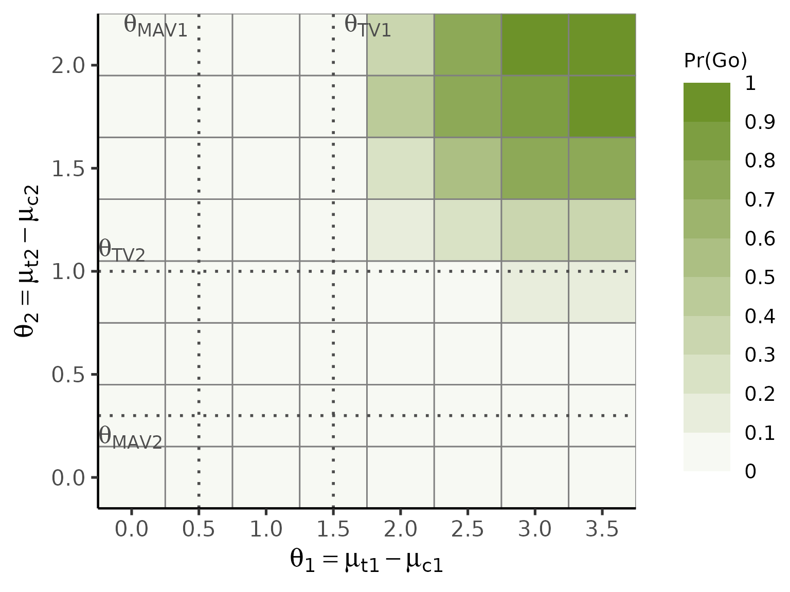

The same function supports design = 'uncontrolled' (with hypothetical control mean mu0_c and scale factor r) and design = 'external' (with power prior arguments ne_c, bar_ye_c, se_c, alpha0e_c). The argument prob = 'predictive' switches to predictive probability (with future sample sizes m_t, m_c and null thresholds theta_NULL1, theta_NULL2). The function signature and output format are identical across all combinations.

---

6. Optimal Threshold Search

6.1 Objective and Algorithm

Because there are two decision thresholds $(\gamma_1, \gamma_2)$, the optimal search is performed over a two-dimensional grid $\Gamma_1 \times \Gamma_2$ (arguments gamma_go_grid and gamma_nogo_grid). The two thresholds are calibrated independently under separate scenarios:

• $\gamma_1^*$: calibrated under the Go-calibration scenario (mu_t_go, Sigma_t_go, mu_c_go, Sigma_c_go; typically the null scenario $\boldsymbol{\mu}_t = \boldsymbol{\mu}_c$), so that $\Pr(\mathrm{Go}) < \texttt{target\_go}$.
• $\gamma_2^*$: calibrated under the NoGo-calibration scenario (mu_t_nogo, Sigma_t_nogo, mu_c_nogo, Sigma_c_nogo; typically the alternative scenario), so that $\Pr(\mathrm{NoGo}) < \texttt{target\_nogo}$.

getgamma2cont() uses a three-stage strategy:

Stage 1 (Simulate and precompute): $n_\mathrm{sim}$ bivariate datasets are generated separately from each calibration scenario. For each replicate $i$, pbayespostpred2cont() is called once in vectorised mode to return the full region probability vector. The marginal Go and NoGo probabilities per replicate are:

$$\hat{g}_{\mathrm{Go},i} = \sum_{\ell \in \text{GoRegions}} \hat{p}_{i\ell}, \qquad \hat{g}_{\mathrm{NoGo},i} = \sum_{\ell \in \text{NoGoRegions}} \hat{p}_{i\ell}.$$

Stage 2 (Gamma sweep): For each candidate $\gamma_1 \in \Gamma_1$ (under the Go-calibration scenario) and each $\gamma_2 \in \Gamma_2$ (under the NoGo-calibration scenario):

$$\Pr(\mathrm{Go} \mid \gamma_1) = \frac{1}{n_\mathrm{sim}} \sum_{i=1}^{n_\mathrm{sim}} \mathbf{1}\!\left[\hat{g}_{\mathrm{Go},i} \ge \gamma_1\right],$$

$$\Pr(\mathrm{NoGo} \mid \gamma_2) = \frac{1}{n_\mathrm{sim}} \sum_{i=1}^{n_\mathrm{sim}} \mathbf{1}\!\left[\hat{g}_{\mathrm{NoGo},i} \ge \gamma_2\right].$$

The results are stored as vectors PrGo_grid and PrNoGo_grid indexed by gamma_go_grid and gamma_nogo_grid, respectively.

Stage 3 (Optimal selection): $\gamma_1^*$ is the smallest grid value satisfying $\Pr(\mathrm{Go} \mid \gamma_1) < \texttt{target\_go}$; $\gamma_2^*$ is the smallest grid value satisfying $\Pr(\mathrm{NoGo} \mid \gamma_2) < \texttt{target\_nogo}$.

6.2 Example: Controlled Design, Posterior Probability

Go-calibration scenario: $\boldsymbol{\mu}_t = (0.5, 0.3)^\top$, $\boldsymbol{\mu}_c = (0, 0)^\top$ (effect at MAV boundary – above which Go is not yet warranted, so $\Pr(\mathrm{Go}) < \texttt{target\_go}$ is required). NoGo-calibration scenario: $\boldsymbol{\mu}_t = (1.0, 0.6)^\top$, $\boldsymbol{\mu}_c = (0, 0)^\top$ (effect between MAV and TV – above which NoGo should be unlikely).

res_gamma <- getgamma2cont(
  nsim = 500L, prob = 'posterior', design = 'controlled',
  prior = 'vague',
  GoRegions = 1L, NoGoRegions = 9L,
  mu_t_go    = c(0.5, 0.3), Sigma_t_go    = Sigma,
  mu_c_go    = c(0.0, 0.0), Sigma_c_go    = Sigma,
  mu_t_nogo  = c(1.0, 0.6), Sigma_t_nogo  = Sigma,
  mu_c_nogo  = c(0.0, 0.0), Sigma_c_nogo  = Sigma,
  target_go = 0.05, target_nogo = 0.20,
  n_t = 20L, n_c = 20L,
  theta_TV1  = 1.5, theta_MAV1 = 0.5,
  theta_TV2  = 1.0, theta_MAV2 = 0.3,
  theta_NULL1 = NULL, theta_NULL2 = NULL,
  m_t = NULL, m_c = NULL,
  kappa0_t = NULL, nu0_t = NULL, mu0_t = NULL, Lambda0_t = NULL,
  kappa0_c = NULL, nu0_c = NULL, mu0_c = NULL, Lambda0_c = NULL,
  r = NULL,
  ne_t = NULL, ne_c = NULL, alpha0e_t = NULL, alpha0e_c = NULL,
  bar_ye_t = NULL, bar_ye_c = NULL, se_t = NULL, se_c = NULL,
  nMC = 500L, CalcMethod = 'MC',
  gamma_go_grid   = seq(0.05, 0.95, by = 0.05),
  gamma_nogo_grid = seq(0.05, 0.95, by = 0.05),
  seed = 42L
)
plot(res_gamma, base_size = 20)

The same function supports design = 'uncontrolled' (with mu0_c and r) and design = 'external' (with power prior arguments ne_c, bar_ye_c, se_c, alpha0e_c). Setting prob = 'predictive' switches to predictive probability calibration (with theta_NULL1, theta_NULL2, m_t, m_c). The function signature is identical across all combinations.

---

7. Summary

This vignette covered two continuous endpoint analysis in BayesianQDM:

1. Bayesian model: NIW conjugate posterior with explicit update formulae for $\kappa_{nj}$, $\nu_{nj}$, $\boldsymbol{\mu}_{nj}$, and $\Lambda_{nj}$; bivariate non-standardised $t$ marginal posterior.
2. Nine-region grid for posterior probability and four-region grid for predictive probability; typical choice Go = R1, NoGo = R9 (posterior) or R4 (predictive).
3. Two computation methods: MC (vectorised pre-generated draws with Cholesky reuse) and MM (Mahalanobis-distance fourth-moment matching via Yamaguchi et al. (2025), Theorem 3, + mvtnorm::pmvt for joint probability; requires $\nu_j > 4$).
4. Three study designs: controlled, uncontrolled ($\boldsymbol{\mu}_{0c}$ and $r$ fixed), external design (vague power prior follows Corollary 2 of Huang et al. (2025); NIW power prior follows Theorems 5–6).
5. Operating characteristics: Monte Carlo estimation with vectorised region probability computation.
6. Optimal threshold search: three-stage strategy in getgamma2cont() calibrating $\gamma_1^*$ and $\gamma_2^*$ independently under separate Go- and NoGo-calibration scenarios, with calibration curves visualised via plot() and optimal thresholds marked at the target probability levels ($\Pr(\mathrm{Go}) < 0.05$ under null, $\Pr(\mathrm{NoGo}) < 0.20$ under alternative).

See vignette("two-binary") for the analogous two binary endpoint analysis.