Single Continuous Endpoint

Motivating Scenario

We use a hypothetical Phase IIa proof-of-concept (PoC) trial in moderate-to-severe rheumatoid arthritis (RA). The investigational drug is compared with placebo in a 1:1 randomised controlled trial with $n_t = n_c = 15$ patients per group.

Endpoint: change from baseline in DAS28 score (a larger decrease indicates greater improvement).

Clinically meaningful thresholds (posterior probability):

• Target Value ($\theta_{\mathrm{TV}}$) = 1.5 (ambitious target)
• Minimum Acceptable Value ($\theta_{\mathrm{MAV}}$) = 0.5 (lower bar)

Null hypothesis threshold (predictive probability): $\theta_{\mathrm{NULL}} = 1.0$.

Decision thresholds: $\gamma_{\mathrm{go}} = 0.80$ (Go), $\gamma_{\mathrm{nogo}} = 0.20$ (NoGo).

Observed data (used in Sections 2–4): $\bar{y}_t = 3.2$, $s_t = 2.0$ (treatment); $\bar{y}_c = 1.1$, $s_c = 1.8$ (control).

---

1. Bayesian Model: Normal-Inverse-Chi-Squared Conjugate

1.1 Prior Distribution

For group $j$ ($j = t$: treatment, $j = c$: control), patient $i$ ($i = 1, \ldots, n_j$), we model the continuous outcome as

$$y_{ij} \mid \mu_j, \sigma_j^2 \;\overset{iid}{\sim}\; \mathcal{N}(\mu_j,\, \sigma_j^2).$$

The conjugate prior is the Normal-Inverse-Chi-squared (N-Inv-$\chi^2$) distribution:

$$(\mu_j,\, \sigma_j^2) \;\sim\; \mathrm{N\text{-}Inv\text{-}\chi^2} \!\left(\mu_{0j},\, \kappa_{0j},\, \nu_{0j},\, \sigma_{0j}^2\right),$$

where $\mu_{0j}$ (mu0_t, mu0_c) is the prior mean, $\kappa_{0j}$ (kappa0_t, kappa0_c) $> 0$ the prior precision (pseudo-sample size), $\nu_{0j}$ (nu0_t, nu0_c) $> 0$ the prior degrees of freedom, and $\sigma_{0j}^2$ (sigma0_t, sigma0_c) $> 0$ the prior scale.

The vague (Jeffreys) prior is obtained by letting $\kappa_{0j} \to 0$ and $\nu_{0j} \to 0$, which places minimal information on the parameters.

1.2 Posterior Distribution

Given $n_j$ observations with sample mean $\bar{y}_j$ and sample standard deviation $s_j$, the posterior parameters are updated as follows:

$$\kappa_{nj} = \kappa_{0j} + n_j, \qquad \nu_{nj} = \nu_{0j} + n_j,$$

$$\mu_{nj} = \frac{\kappa_{0j}\,\mu_{0j} + n_j\,\bar{y}_j}{\kappa_{nj}},$$

$$\sigma_{nj}^2 = \frac{\nu_{0j}\,\sigma_{0j}^2 + (n_j - 1)\,s_j^2 + \dfrac{n_j\,\kappa_{0j}}{\kappa_{nj}}\,(\mu_{0j} - \bar{y}_j)^2} {\nu_{nj}}.$$

The marginal posterior of the group mean $\mu_j$ is a non-standardised $t$-distribution:

$$\mu_j \mid \mathbf{y}_j \;\sim\; t_{\nu_{nj}}\!\!\left(\mu_{nj},\; \frac{\sigma_{nj}}{\sqrt{\kappa_{nj}}}\right).$$

Under the vague prior ($\kappa_{0j} = \nu_{0j} = 0$), this simplifies to

$$\mu_j \mid \mathbf{y}_j \;\sim\; t_{n_j - 1}\!\!\left(\bar{y}_j,\; \frac{s_j}{\sqrt{n_j}}\right).$$

1.3 Posterior of the Treatment Effect

The treatment effect is $\theta = \mu_t - \mu_c$. Since the two groups are independent, the posterior of $\theta$ is the distribution of the difference of two independent non-standardised $t$-variables:

$$T_j \;\sim\; t_{\nu_{nj}}(\mu_{nj},\, \sigma_{nj}^{\dagger}), \qquad j = t, c,$$

where the posterior scale is $\sigma_{nj}^{\dagger} = \sigma_{nj} / \sqrt{\kappa_{nj}}$.

The posterior probability that $\theta$ exceeds a threshold $\theta_0$,

$$P(\theta > \theta_0 \mid \mathbf{y}) = P(T_t - T_c > \theta_0),$$

is computed by one of three methods described in Section 3.

---

2. Posterior Predictive Probability

2.1 Predictive Distribution

Let $\bar{\tilde{y}}_j$ denote the future sample mean based on $m_j$ future patients. Under the N-Inv-$\chi^2$ posterior, the predictive distribution of $\bar{\tilde{y}}_j$ is again a non-standardised $t$-distribution:

$$\bar{\tilde{y}}_j \mid \mathbf{y}_j \;\sim\; t_{\nu_{nj}}\!\!\left(\mu_{nj},\; \sigma_{nj}\sqrt{\frac{1 + \kappa_{nj}}{\kappa_{nj}\, m_j}}\right).$$

Under the vague prior ($\kappa_{nj} = n_j$, $\sigma_{nj} = s_j$) this becomes

$$\bar{\tilde{y}}_j \mid \mathbf{y}_j \;\sim\; t_{n_j - 1}\!\!\left(\bar{y}_j,\; s_j\sqrt{\frac{n_j + 1}{n_j\, m_j}}\right).$$

2.2 Posterior Predictive Probability

The posterior predictive probability that the future treatment effect exceeds the null threshold $\theta_{\mathrm{NULL}}$ is

$$P\!\left(\bar{\tilde{y}}_t - \bar{\tilde{y}}_c > \theta_{\mathrm{NULL}} \mid \mathbf{y}\right),$$

computed by the same three methods as the posterior probability but with the predictive scale replacing the posterior scale.

---

3. Three Computation Methods

3.1 Numerical Integration (NI)

The exact CDF of $D = T_t - T_c$ is expressed as a one-dimensional integral:

$$P(D \le \theta_0) = \int_{-\infty}^{\infty} F_{t_{\nu_c}(\mu_c, \sigma_c)}\!\left(t - \theta_0\right)\, f_{t_{\nu_t}(\mu_t, \sigma_t)}(t)\; dt,$$

where $F_{t_\nu(\mu,\sigma)}$ and $f_{t_\nu(\mu,\sigma)}$ are the CDF and PDF of the non-standardised $t$-distribution respectively. This integral is evaluated by stats::integrate() (adaptive Gauss-Kronrod quadrature) in ptdiff_NI(). The method is exact but evaluates the integral once per call and is therefore slow for large-scale simulation.

3.2 Monte Carlo Simulation (MC)

$n_{\mathrm{MC}}$ independent samples are drawn from each marginal:

$$T_t^{(i)} \;\sim\; t_{\nu_t}(\mu_t, \sigma_t), \quad T_c^{(i)} \;\sim\; t_{\nu_c}(\mu_c, \sigma_c), \quad i = 1, \ldots, n_{\mathrm{MC}},$$

and the probability is estimated as

$$\widehat{P}(D > \theta_0) = \frac{1}{n_{\mathrm{MC}}} \sum_{i=1}^{n_{\mathrm{MC}}} \mathbf{1}\!\left[T_t^{(i)} - T_c^{(i)} > \theta_0\right].$$

When called from pbayesdecisionprob1cont() with $n_{\mathrm{sim}}$ simulation replicates, all draws are generated as a single $n_{\mathrm{MC}} \times n_{\mathrm{sim}}$ matrix to avoid loop overhead.

3.3 Moment-Matching Approximation (MM)

The difference $D = T_t - T_c$ is approximated by a single non-standardised $t$-distribution (Yamaguchi et al., 2025, Theorem 1). Let

$$Q^*_u = \left(\sigma_t^2\,\frac{\nu_t}{\nu_t - 2} + \sigma_c^2\,\frac{\nu_c}{\nu_c - 2}\right)^{\!2},$$

$$Q_u = \frac{(\sigma_t^2)^2\,\nu_t^2}{(\nu_t-2)(\nu_t-4)} + \frac{(\sigma_c^2)^2\,\nu_c^2}{(\nu_c-2)(\nu_c-4)} + 2\left(\sigma_t^2\,\frac{\nu_t}{\nu_t-2}\right) \!\left(\sigma_c^2\,\frac{\nu_c}{\nu_c-2}\right) \qquad (\nu_t > 4,\; \nu_c > 4).$$

Then $D \approx Z^* \sim t_{\nu^*}(\mu^*, \sigma^*)$, where

$$\mu^* = \mu_t - \mu_c,$$

$$\nu^* = \frac{2Q^*_u - 4Q_u}{Q^*_u - Q_u},$$

$$\sigma^* = \sqrt{\left(\sigma_t^2\,\frac{\nu_t}{\nu_t - 2} + \sigma_c^2\,\frac{\nu_c}{\nu_c - 2}\right) \frac{\nu^* - 2}{\nu^*}}.$$

The CDF is evaluated via a single call to stats::pt(). This method requires $\nu_j > 4$, is exact in the normal limit ($\nu_j \to \infty$), and is fully vectorised — making it the recommended method for large-scale simulation.

3.4 Comparison of the Three Methods

# Observed data (nMC excluded from base list; passed individually per method)
args_base <- list(
  prob = 'posterior', design = 'controlled', prior = 'vague',
  theta0 = 1.0,
  n_t = 15, n_c = 15,
  bar_y_t = 3.2, s_t = 2.0,
  bar_y_c = 1.1, s_c = 1.8,
  m_t = NULL, m_c = NULL,
  kappa0_t = NULL, kappa0_c = NULL, nu0_t = NULL, nu0_c = NULL,
  mu0_t = NULL, mu0_c = NULL, sigma0_t = NULL, sigma0_c = NULL,
  r = NULL,
  ne_t = NULL, ne_c = NULL, alpha0e_t = NULL, alpha0e_c = NULL,
  bar_ye_t = NULL, se_t = NULL, bar_ye_c = NULL, se_c = NULL
)

p_ni <- do.call(pbayespostpred1cont,
                c(args_base, list(CalcMethod = 'NI', nMC = NULL)))
p_mm <- do.call(pbayespostpred1cont,
                c(args_base, list(CalcMethod = 'MM', nMC = NULL)))
set.seed(42)
p_mc <- do.call(pbayespostpred1cont,
                c(args_base, list(CalcMethod = 'MC', nMC = 10000L)))

cat(sprintf("NI : %.6f  (exact)\n",      p_ni))
#> NI : 0.069397  (exact)
cat(sprintf("MM : %.6f  (approx)\n",     p_mm))
#> MM : 0.069397  (approx)
cat(sprintf("MC : %.6f  (n_MC=10000)\n", p_mc))
#> MC : 0.073400  (n_MC=10000)

---

4. Study Designs

4.1 Controlled Design

Standard parallel-group RCT with observed data from both treatment ($n_t$, $\bar{y}_t$, $s_t$) and control ($n_c$, $\bar{y}_c$, $s_c$) groups. Both posteriors are updated from the PoC data.

Vague prior — posterior probability:

# P(mu_t - mu_c > theta_TV | data) and P(mu_t - mu_c <= theta_MAV | data)
p_tv <- pbayespostpred1cont(
  prob = 'posterior', design = 'controlled', prior = 'vague',
  CalcMethod = 'NI', theta0 = 1.5, nMC = NULL,
  n_t = 15, n_c = 15,
  bar_y_t = 3.2, s_t = 2.0,
  bar_y_c = 1.1, s_c = 1.8,
  m_t = NULL, m_c = NULL,
  kappa0_t = NULL, kappa0_c = NULL, nu0_t = NULL, nu0_c = NULL,
  mu0_t = NULL, mu0_c = NULL, sigma0_t = NULL, sigma0_c = NULL,
  r = NULL,
  ne_t = NULL, ne_c = NULL, alpha0e_t = NULL, alpha0e_c = NULL,
  bar_ye_t = NULL, se_t = NULL, bar_ye_c = NULL, se_c = NULL,
  lower.tail = FALSE
)

p_mav <- pbayespostpred1cont(
  prob = 'posterior', design = 'controlled', prior = 'vague',
  CalcMethod = 'NI', theta0 = 0.5, nMC = NULL,
  n_t = 15, n_c = 15,
  bar_y_t = 3.2, s_t = 2.0,
  bar_y_c = 1.1, s_c = 1.8,
  m_t = NULL, m_c = NULL,
  kappa0_t = NULL, kappa0_c = NULL, nu0_t = NULL, nu0_c = NULL,
  mu0_t = NULL, mu0_c = NULL, sigma0_t = NULL, sigma0_c = NULL,
  r = NULL,
  ne_t = NULL, ne_c = NULL, alpha0e_t = NULL, alpha0e_c = NULL,
  bar_ye_t = NULL, se_t = NULL, bar_ye_c = NULL, se_c = NULL,
  lower.tail = FALSE
)

cat(sprintf("P(theta > theta_TV  | data) = %.4f  -> Go  criterion: >= 0.80? %s\n",
            p_tv, ifelse(p_tv >= 0.80, "YES", "NO")))
#> P(theta > theta_TV  | data) = 0.7940  -> Go  criterion: >= 0.80? NO
cat(sprintf("P(theta <= theta_MAV | data) = %.4f  -> NoGo criterion: >= 0.20? %s\n",
            1 - p_mav, ifelse((1 - p_mav) >= 0.20, "YES", "NO")))
#> P(theta <= theta_MAV | data) = 0.0178  -> NoGo criterion: >= 0.20? NO
cat(sprintf("Decision: %s\n",
            ifelse(p_tv >= 0.80 & (1 - p_mav) < 0.20, "Go",
                   ifelse(p_tv < 0.80 & (1 - p_mav) >= 0.20, "NoGo",
                          ifelse(p_tv >= 0.80 & (1 - p_mav) >= 0.20, "Miss", "Gray")))))
#> Decision: Gray

N-Inv-$\chi^2$ informative prior:

Historical knowledge suggests treatment mean $\sim 3.0$ and control mean $\sim 1.0$ with prior pseudo-sample size $\kappa_{0t} = \kappa_{0c} = 5$ (kappa0_t, kappa0_c) and degrees of freedom $\nu_{0t} = \nu_{0c} = 5$ (nu0_t, nu0_c).

p_tv_inf <- pbayespostpred1cont(
  prob = 'posterior', design = 'controlled', prior = 'N-Inv-Chisq',
  CalcMethod = 'NI', theta0 = 1.5, nMC = NULL,
  n_t = 15, n_c = 15,
  bar_y_t = 3.2, s_t = 2.0,
  bar_y_c = 1.1, s_c = 1.8,
  m_t = NULL, m_c = NULL,
  kappa0_t = 5, kappa0_c = 5,
  nu0_t    = 5, nu0_c    = 5,
  mu0_t    = 3.0, mu0_c  = 1.0,
  sigma0_t = 2.0, sigma0_c = 1.8,
  r = NULL,
  ne_t = NULL, ne_c = NULL, alpha0e_t = NULL, alpha0e_c = NULL,
  bar_ye_t = NULL, se_t = NULL, bar_ye_c = NULL, se_c = NULL,
  lower.tail = FALSE
)
cat(sprintf("P(theta > theta_TV | data, N-Inv-Chisq prior) = %.4f\n", p_tv_inf))
#> P(theta > theta_TV | data, N-Inv-Chisq prior) = 0.8274

Posterior predictive probability (future Phase III: $m_t = m_c = 60$):

p_pred <- pbayespostpred1cont(
  prob = 'predictive', design = 'controlled', prior = 'vague',
  CalcMethod = 'NI', theta0 = 1.0, nMC = NULL,
  n_t = 15, n_c = 15, m_t = 60, m_c = 60,
  bar_y_t = 3.2, s_t = 2.0,
  bar_y_c = 1.1, s_c = 1.8,
  kappa0_t = NULL, kappa0_c = NULL, nu0_t = NULL, nu0_c = NULL,
  mu0_t = NULL, mu0_c = NULL, sigma0_t = NULL, sigma0_c = NULL,
  r = NULL,
  ne_t = NULL, ne_c = NULL, alpha0e_t = NULL, alpha0e_c = NULL,
  bar_ye_t = NULL, se_t = NULL, bar_ye_c = NULL, se_c = NULL,
  lower.tail = FALSE
)
cat(sprintf("Predictive probability (m_t = m_c = 60) = %.4f\n", p_pred))
#> Predictive probability (m_t = m_c = 60) = 0.9966

4.2 Uncontrolled Design (Single-Arm)

When no concurrent control group is enrolled, the control distribution is specified from external knowledge:

• Hypothetical control mean: $\mu_{0c}$ (mu0_c, fixed scalar)
• Variance scaling: $\sigma_c = \sqrt{r} \cdot \sigma_t$, so $r = 1$ assumes equal variances

The posterior of the control mean is not updated from observed data; only the treatment posterior is updated.

p_unctrl <- pbayespostpred1cont(
  prob = 'posterior', design = 'uncontrolled', prior = 'vague',
  CalcMethod = 'MM', theta0 = 1.5, nMC = NULL,
  n_t = 15, n_c = NULL,
  bar_y_t = 3.2, s_t = 2.0,
  bar_y_c = NULL, s_c = NULL,
  m_t = NULL, m_c = NULL,
  kappa0_t = NULL, kappa0_c = NULL, nu0_t = NULL, nu0_c = NULL,
  mu0_t = NULL, mu0_c = 1.0,   # hypothetical control mean
  sigma0_t = NULL, sigma0_c = NULL,
  r = 1.0,                     # equal variance assumption
  ne_t = NULL, ne_c = NULL, alpha0e_t = NULL, alpha0e_c = NULL,
  bar_ye_t = NULL, se_t = NULL, bar_ye_c = NULL, se_c = NULL,
  lower.tail = FALSE
)
cat(sprintf("P(theta > theta_TV | data, uncontrolled) = %.4f\n", p_unctrl))
#> P(theta > theta_TV | data, uncontrolled) = 0.8184

4.3 External Design (Power Prior)

In the external design, historical data from a prior study are incorporated via a power prior with borrowing weight $\alpha_{0e} \in (0, 1]$. The two prior specifications yield different posterior update formulae.

Vague prior (prior = 'vague')

For group $j$ with $n_{e,j}$ external patients, external mean $\bar{y}_{e,j}$, and external SD $s_{e,j}$, the posterior parameters after combining the power prior with the PoC data are given by Theorem 4 of Huang et al. (2025):

$$\mu_{nj}^* = \frac{\alpha_{0e,j}\, n_{e,j}\, \bar{y}_{e,j} + n_j\, \bar{y}_j} {\alpha_{0e,j}\, n_{e,j} + n_j},$$

$$\kappa_{nj}^* = \alpha_{0e,j}\, n_{e,j} + n_j,$$

$$\nu_{nj}^* = \alpha_{0e,j}\, n_{e,j} + n_j - 1,$$

$$(\sigma_{nj}^*)^2 = \frac{\alpha_{0e,j}(n_{e,j}-1)\, s_{e,j}^2 + (n_j-1)\, s_j^2 + \dfrac{\alpha_{0e,j}\, n_{e,j}\, n_j\, (\bar{y}_{e,j} - \bar{y}_j)^2} {\alpha_{0e,j}\, n_{e,j} + n_j}} {\alpha_{0e,j}\, n_{e,j} + n_j}.$$

The marginal posterior of $\mu_j$ is then

$$\mu_j \mid \mathbf{y}_j \;\sim\; t_{\nu_{nj}^*}\!\!\left(\mu_{nj}^*,\; \frac{\sigma_{nj}^*}{\sqrt{\kappa_{nj}^*}}\right).$$

Setting $\alpha_{0e,j} = 1$ corresponds to full borrowing; as $\alpha_{0e,j} \to 0$ the result recovers the vague-prior posterior from the current data alone.

N-Inv-$\chi^2$ prior (prior = 'N-Inv-Chisq')

When an informative N-Inv-$\chi^2(\mu_{0j}, \kappa_{0j}, \nu_{0j}, \sigma_{0j}^2)$ initial prior is specified, the power prior is first formed by combining the initial prior with the discounted external data (Theorem 1 of Huang et al., 2025):

$$\mu_{e,j} = \frac{\alpha_{0e,j}\, n_{e,j}\, \bar{y}_{e,j} + \kappa_{0j}\, \mu_{0j}} {\alpha_{0e,j}\, n_{e,j} + \kappa_{0j}},$$

$$\kappa_{e,j} = \alpha_{0e,j}\, n_{e,j} + \kappa_{0j},$$

$$\nu_{e,j} = \alpha_{0e,j}\, n_{e,j} + \nu_{0j},$$

$$\sigma_{e,j}^2 = \frac{\alpha_{0e,j}(n_{e,j}-1)\, s_{e,j}^2 + \nu_{0j}\, \sigma_{0j}^2 + \dfrac{\alpha_{0e,j}\, n_{e,j}\, \kappa_{0j}\, (\bar{y}_{e,j} - \mu_{0j})^2} {\alpha_{0e,j}\, n_{e,j} + \kappa_{0j}}} {\nu_{e,j}}.$$

This intermediate result is then updated with the PoC data by standard conjugate updating (Theorem 2 of Huang et al., 2025):

$$\mu_{nj}^* = \frac{\kappa_{e,j}\, \mu_{e,j} + n_j\, \bar{y}_j} {\kappa_{e,j} + n_j},$$

$$\kappa_{nj}^* = \kappa_{e,j} + n_j,$$

$$\nu_{nj}^* = \nu_{e,j} + n_j,$$

$$(\sigma_{nj}^*)^2 = \frac{\nu_{e,j}\, \sigma_{e,j}^2 + (n_j-1)\, s_j^2 + \dfrac{n_j\, \kappa_{e,j}\, (\mu_{e,j} - \bar{y}_j)^2} {\kappa_{e,j} + n_j}} {\nu_{nj}^*}.$$

The marginal posterior of $\mu_j$ is then

$$\mu_j \mid \mathbf{y}_j \;\sim\; t_{\nu_{nj}^*}\!\!\left(\mu_{nj}^*,\; \frac{\sigma_{nj}^*}{\sqrt{\kappa_{nj}^*}}\right).$$

Example: external control design, vague prior

Here, $n_{e,c} = 20$ (ne_c), $\bar{y}_{e,c} = 0.9$ (bar_ye_c), $s_{e,c} = 1.8$ (se_c), $\alpha_{0e,c} = 0.5$ (alpha0e_c) (50% borrowing from external control):

p_ext <- pbayespostpred1cont(
  prob = 'posterior', design = 'external', prior = 'vague',
  CalcMethod = 'MM', theta0 = 1.5, nMC = NULL,
  n_t = 15, n_c = 15,
  bar_y_t = 3.2, s_t = 2.0,
  bar_y_c = 1.1, s_c = 1.8,
  m_t = NULL, m_c = NULL,
  kappa0_t = NULL, kappa0_c = NULL, nu0_t = NULL, nu0_c = NULL,
  mu0_t = NULL, mu0_c = NULL, sigma0_t = NULL, sigma0_c = NULL,
  r = NULL,
  ne_t = NULL, ne_c = 20L, alpha0e_t = NULL, alpha0e_c = 0.5,
  bar_ye_t = NULL, se_t = NULL, bar_ye_c = 0.9, se_c = 1.8,
  lower.tail = FALSE
)
cat(sprintf("P(theta > theta_TV | data, external control design, alpha=0.5) = %.4f\n",
            p_ext))
#> P(theta > theta_TV | data, external control design, alpha=0.5) = 0.8517

Effect of the borrowing weight: varying $\alpha_{0e,c}$ from 0 to 1 shows how external data influence the posterior.

# alpha0e_c must be in (0, 1]; start from 0.01 to avoid validation error
alpha_seq <- c(0.01, seq(0.1, 1.0, by = 0.1))
p_alpha   <- sapply(alpha_seq, function(a) {
  pbayespostpred1cont(
    prob = 'posterior', design = 'external', prior = 'vague',
    CalcMethod = 'MM', theta0 = 1.5, nMC = NULL,
    n_t = 15, n_c = 15,
    bar_y_t = 3.2, s_t = 2.0,
    bar_y_c = 1.1, s_c = 1.8,
    m_t = NULL, m_c = NULL,
    kappa0_t = NULL, kappa0_c = NULL, nu0_t = NULL, nu0_c = NULL,
    mu0_t = NULL, mu0_c = NULL, sigma0_t = NULL, sigma0_c = NULL,
    r = NULL,
    ne_t = NULL, ne_c = 20L, alpha0e_t = NULL, alpha0e_c = a,
    bar_ye_t = NULL, se_t = NULL, bar_ye_c = 0.9, se_c = 1.8,
    lower.tail = FALSE
  )
})
data.frame(alpha_ec = alpha_seq, P_gt_TV = round(p_alpha, 4))
#>    alpha_ec P_gt_TV
#> 1      0.01  0.7994
#> 2      0.10  0.8133
#> 3      0.20  0.8259
#> 4      0.30  0.8361
#> 5      0.40  0.8446
#> 6      0.50  0.8517
#> 7      0.60  0.8577
#> 8      0.70  0.8629
#> 9      0.80  0.8674
#> 10     0.90  0.8713
#> 11     1.00  0.8748

---

5. Operating Characteristics

5.1 Definition

For given true parameters $(\mu_t, \mu_c, \sigma_t, \sigma_c)$, the operating characteristics are the probabilities of each decision outcome under the Go/NoGo/Gray/Miss rule with thresholds $(\gamma_{\mathrm{go}}, \gamma_{\mathrm{nogo}})$. These are estimated by Monte Carlo simulation over $n_{\mathrm{sim}}$ replicates:

$$\widehat{\Pr}(\mathrm{Go}) = \frac{1}{n_{\mathrm{sim}}} \sum_{i=1}^{n_{\mathrm{sim}}} \mathbf{1}\!\left[g_{\mathrm{Go}}^{(i)} \ge \gamma_{\mathrm{go}} \;\text{ and }\; g_{\mathrm{NoGo}}^{(i)} < \gamma_{\mathrm{nogo}}\right],$$

$$\widehat{\Pr}(\mathrm{NoGo}) = \frac{1}{n_{\mathrm{sim}}} \sum_{i=1}^{n_{\mathrm{sim}}} \mathbf{1}\!\left[g_{\mathrm{Go}}^{(i)} < \gamma_{\mathrm{go}} \;\text{ and }\; g_{\mathrm{NoGo}}^{(i)} \ge \gamma_{\mathrm{nogo}}\right],$$

$$\widehat{\Pr}(\mathrm{Gray}) = 1 - \widehat{\Pr}(\mathrm{Go}) - \widehat{\Pr}(\mathrm{NoGo}) - \widehat{\Pr}(\mathrm{Miss}),$$

where

$$g_{\mathrm{Go}}^{(i)} = P(\theta > \theta_{\mathrm{TV}} \mid \mathbf{y}^{(i)}), \qquad g_{\mathrm{NoGo}}^{(i)} = P(\theta \le \theta_{\mathrm{MAV}} \mid \mathbf{y}^{(i)})$$

are evaluated for the $i$-th simulated dataset $\mathbf{y}^{(i)}$. A Miss ($g_{\mathrm{Go}} \ge \gamma_{\mathrm{go}}$ AND $g_{\mathrm{NoGo}} \ge \gamma_{\mathrm{nogo}}$) indicates an inconsistent threshold configuration and triggers an error by default (error_if_Miss = TRUE).

5.2 Example: Controlled Design, Posterior Probability

oc_ctrl <- pbayesdecisionprob1cont(
  nsim       = 500L,
  prob       = 'posterior',
  design     = 'controlled',
  prior      = 'vague',
  CalcMethod = 'MM',
  theta_TV   = 1.5,  theta_MAV = 0.5,  theta_NULL = NULL,
  nMC        = NULL,
  gamma_go   = 0.80, gamma_nogo = 0.20,
  n_t = 15,   n_c = 15,
  m_t = NULL, m_c = NULL,
  kappa0_t = NULL, kappa0_c = NULL, nu0_t = NULL, nu0_c = NULL,
  mu0_t = NULL, mu0_c = NULL, sigma0_t = NULL, sigma0_c = NULL,
  mu_t    = seq(1.0, 4.0, by = 0.5),
  mu_c    = 1.0,
  sigma_t = 2.0,
  sigma_c = 2.0,
  r = NULL,
  ne_t = NULL, ne_c = NULL, alpha0e_t = NULL, alpha0e_c = NULL,
  bar_ye_t = NULL, se_t = NULL, bar_ye_c = NULL, se_c = NULL,
  error_if_Miss = TRUE, Gray_inc_Miss = FALSE,
  seed = 42L
)
print(oc_ctrl)
#> Go/NoGo/Gray Decision Probabilities (Single Continuous Endpoint) 
#> ---------------------------------------------------------------- 
#>   Probability type : posterior 
#>   Design           : controlled 
#>   Prior            : vague 
#>   Calc method      : MM 
#>   Simulations      : nsim = 500 
#>   Threshold(s)     : TV = 1.5, MAV = 0.5 
#>   Go  threshold    : gamma_go = 0.8 
#>   NoGo threshold   : gamma_nogo = 0.2 
#>   Sample size      : n_t = 15, n_c = 15 
#>   True SD          : sigma_t = 2, sigma_c = 2 
#>   Miss handling    : error_if_Miss = TRUE, Gray_inc_Miss = FALSE 
#>   Seed             : 42 
#> ---------------------------------------------------------------- 
#>  mu_t mu_c    Go  Gray  NoGo
#>   1.0    1 0.002 0.064 0.934
#>   1.5    1 0.014 0.168 0.818
#>   2.0    1 0.066 0.352 0.582
#>   2.5    1 0.182 0.502 0.316
#>   3.0    1 0.418 0.460 0.122
#>   3.5    1 0.684 0.288 0.028
#>   4.0    1 0.878 0.118 0.004
#> ----------------------------------------------------------------
plot(oc_ctrl, base_size = 20)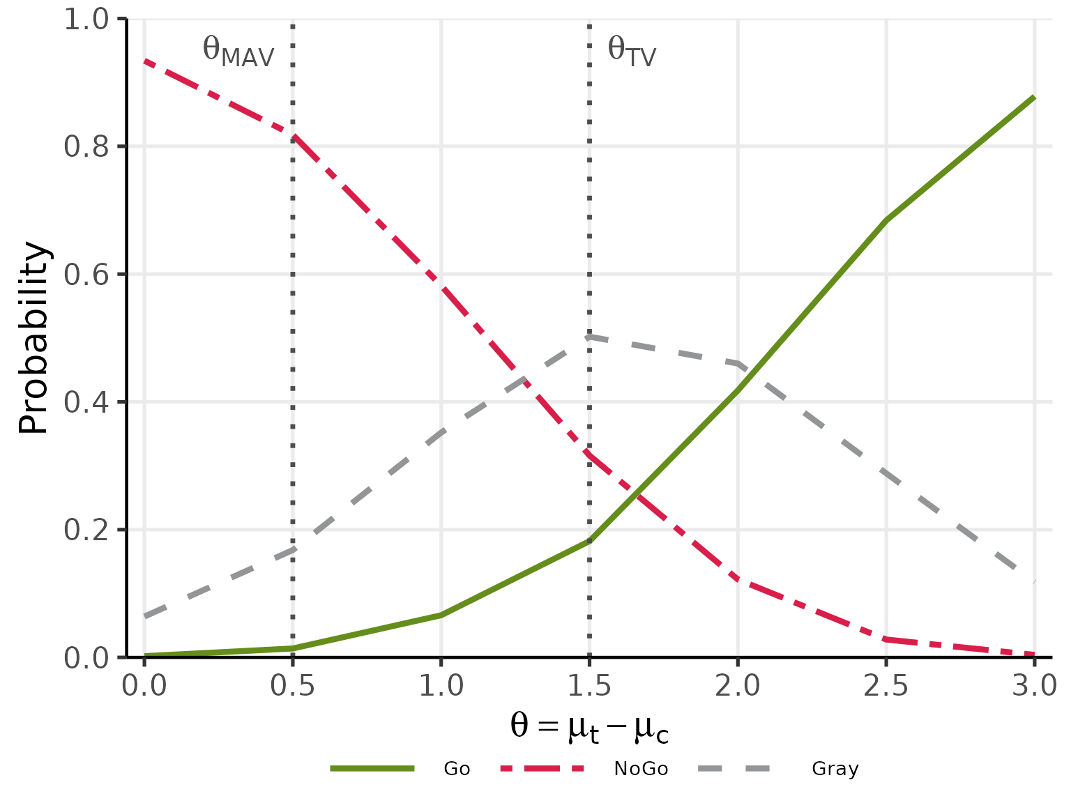

The same function supports design = 'uncontrolled' (with arguments mu0_c and r), design = 'external' (with power prior arguments ne_c, alpha0e_c, bar_ye_c, se_c), and prob = 'predictive' (with future sample size arguments m_t, m_c and theta_NULL). The function signature and output format are identical across all combinations.

---

6. Optimal Threshold Search

6.1 Objective

The getgamma1cont() function finds the optimal pair $(\gamma_{\mathrm{go}}^*, \gamma_{\mathrm{nogo}}^*)$ by grid search over $\Gamma = \{\gamma^{(1)}, \ldots, \gamma^{(K)}\} \subset (0, 1)$. The two thresholds are calibrated independently under separate scenarios:

• $\gamma_{\mathrm{go}}^*$: selected so that $\Pr(\mathrm{Go} \mid \gamma_{\mathrm{go}}^*)$ satisfies a criterion against a target value (e.g., $\Pr(\mathrm{Go}) < 0.05$) under the Go-calibration scenario (mu_t_go, mu_c_go, sigma_t_go, sigma_c_go; typically the null scenario $\mu_t = \mu_c$).
• $\gamma_{\mathrm{nogo}}^*$: selected so that $\Pr(\mathrm{NoGo} \mid \gamma_{\mathrm{nogo}}^*)$ satisfies a criterion (e.g., $\Pr(\mathrm{NoGo}) < 0.20$) under the NoGo-calibration scenario (mu_t_nogo, mu_c_nogo, sigma_t_nogo, sigma_c_nogo; typically the alternative scenario).

The search uses a two-stage strategy:

Stage 1 (Simulate once): $n_{\mathrm{sim}}$ datasets are generated from the true parameter distribution and the probabilities $g_{\mathrm{Go}}^{(i)}$ and $g_{\mathrm{NoGo}}^{(i)}$ are computed for each replicate — independently of $\gamma$.

Stage 2 (Sweep over $\Gamma$): for each candidate $\gamma \in \Gamma$, $\Pr(\mathrm{Go} \mid \gamma)$ and $\Pr(\mathrm{NoGo} \mid \gamma)$ are computed as empirical proportions over the precomputed indicator values without further probability evaluations.

6.2 Example: Controlled Design, Posterior Probability

res_gamma <- getgamma1cont(
  nsim       = 1000L,
  prob       = 'posterior',
  design     = 'controlled',
  prior      = 'vague',
  CalcMethod = 'MM',
  theta_TV   = 1.5, theta_MAV = 0.5, theta_NULL = NULL,
  nMC        = NULL,
  mu_t_go    = 1.0, mu_c_go    = 1.0,   # null scenario: no treatment effect
  sigma_t_go = 2.0, sigma_c_go = 2.0,
  mu_t_nogo    = 2.5, mu_c_nogo    = 1.0,
  sigma_t_nogo = 2.0, sigma_c_nogo = 2.0,
  target_go = 0.05, target_nogo = 0.20,
  n_t = 15L, n_c = 15L, m_t = NULL, m_c = NULL,
  kappa0_t = NULL, kappa0_c = NULL, nu0_t = NULL, nu0_c = NULL,
  mu0_t = NULL, mu0_c = NULL, sigma0_t = NULL, sigma0_c = NULL,
  r = NULL,
  ne_t = NULL, ne_c = NULL, alpha0e_t = NULL, alpha0e_c = NULL,
  bar_ye_t = NULL, bar_ye_c = NULL, se_t = NULL, se_c = NULL,
  gamma_grid = seq(0.01, 0.99, by = 0.01),
  seed = 42L
)
plot(res_gamma, base_size = 20)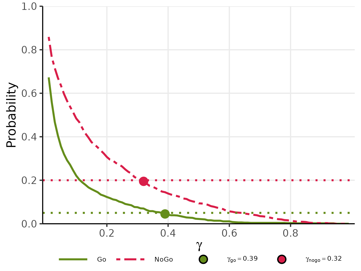

The same function supports design = 'uncontrolled' (with mu_t_go, mu_t_nogo, mu0_c, and r; set mu_c_go and mu_c_nogo to NULL), design = 'external' (with power prior arguments), and prob = 'predictive' (with theta_NULL, m_t, and m_c). The calibration plot and the returned gamma_go/gamma_nogo values are available for all combinations.

---

7. Summary

This vignette covered single continuous endpoint analysis in BayesianQDM:

1. Bayesian model: N-Inv-$\chi^2$ conjugate posterior (vague and informative priors) with explicit update formulae for $\kappa_{nj}$, $\nu_{nj}$, $\mu_{nj}$, and $\sigma_{nj}^2$.
2. Posterior and predictive distributions: marginal $t$-distributions for $\mu_j$ and $\bar{\tilde{y}}_j$, with explicit scale expressions.
3. Three computation methods: NI (exact), MC (simulation), MM (moment-matching approximation; Yamaguchi et al., 2025, Theorem 1); MM requires $\nu_j > 4$ and is recommended for large-scale simulation.
4. Three study designs: controlled (both groups observed), uncontrolled ($\mu_{0c}$ and $r$ fixed from prior knowledge), external design (power prior with borrowing weight $\alpha_{0e,j}$; vague prior follows Theorem 4 of Huang et al. (2025), N-Inv-$\chi^2$ prior follows Theorems 1–2 of Huang et al. (2025)).
5. Operating characteristics: Monte Carlo estimation of $\Pr(\mathrm{Go})$, $\Pr(\mathrm{NoGo})$, $\Pr(\mathrm{Gray})$ across true parameter scenarios.
6. Optimal threshold search: two-stage precompute-then-sweep strategy in getgamma1cont() with user-specified criteria and selection rules.

See vignette("single-binary") for the analogous binary endpoint analysis.