Stratified Designs

library(bbssr)

Design and notation

A trial is stratified into $J \ge 2$ strata, for example by centre or by a baseline factor, and stratum $j$ has $N_{1j}$ patients in group 1 and $N_{2j}$ in group 2, both fixed by the design (random sizes are treated in Random stratum and group sizes). Let $x_{1j}$ and $x_{2j}$ be the numbers of responders of the two groups and $z_j = x_{1j} + x_{2j}$ the number of responders of the stratum. All tests of the Strat* functions use $S = \sum_j x_{1j}$ , the number of responders of group 1 summed over the strata. Given $z = (z_1, \ldots, z_J)$ , the null expectation of $S$ is $E = \sum_j N_{1j} z_j / N_j$ with $N_j = N_{1j} + N_{2j}$ , and each test rejects when $S$ is at most a lower or at least an upper critical value.

The functions follow those for two independent groups: StratRR(), StratPower() and StratSampleSize() for the fixed design, and StratPowerBSSR(), StratGridBSSR(), StratBSSR(), StratTypeIErrorBSSR() and StratAlphaAdjBSSR() for blinded sample size re-estimation.

Tests

Five stratified tests are available. 'CMH' is the Cochran-Mantel-Haenszel statistic $(S - E) / \sqrt{V}$ with the hypergeometric variance $V = \sum_j N_{1j} N_{2j} z_j (N_j - z_j) / \{N_j^2 (N_j - 1)\}$ , and 'Cochran' is Cochran’s statistic with the binomial variance $\sum_j N_{1j} N_{2j} z_j (N_j - z_j) / N_j^3$ , the statistic of Woolson et al. (1986). 'CMH-cc' and 'Cochran-cc' reduce $|S - E|$ by 0.5 when it is at least 0.5, the continuity correction of stats::mantelhaen.test(). Nam (1992) reduces $S - E$ by 0.5 in every outcome; the two corrections reject the same outcomes at one-sided levels up to 0.078, since an outcome with $|S - E| < 0.5$ has a larger one-sided p-value. 'Strat-Fisher' is the stratified exact conditional test of Jung (2014), which refers $S$ to its distribution given $z$ , the convolution of the hypergeometric distributions of the strata. Three unstratified tests, which analyse the table of totals and ignore the strata, are available for comparison (see Analyses that ignore the strata).

Jung (2014, Table 2) analyses the response to thymosin in three strata of patients with bronchogenic carcinoma.

thymosin <- array(c(10, 12, 1, 1, 9, 11, 0, 1, 8, 7, 0, 3), c(2, 2, 3))
p.exact <- stats::mantelhaen.test(thymosin, alternative = 'greater', exact = TRUE)$p.value
p.mh <- stats::mantelhaen.test(thymosin, alternative = 'greater', correct = FALSE)$p.value
round(c(exact = p.exact, mh = p.mh), 4)
#>  exact     mh 
#> 0.1563 0.0760

The one-sided p-values 0.1563 and 0.0760 are those of Jung (2014) for the stratified exact test and the Mantel-Haenszel test, which 'Strat-Fisher' and 'CMH' compute in the same way. StratRR() lists the critical values of a design for every vector of stratum totals.

rr <- StratRR(N1 = c(10, 12), N2 = c(10, 12), alpha = 0.025, Test = 'Strat-Fisher')
print(rr, n = 6)
#> Rejection region of a stratified test
#> 
#>   Test             : Strat-Fisher
#>   Alternative      : greater
#>   Group sizes      : N1 = (10, 12), N2 = (10, 12)
#>   Alpha            : 0.025
#>   Combinations     : 525, of which 457 have a rejected value of S
#> 
#>  z.S1 z.S2 S.min S.max lower upper
#>     5    0     0     5    NA     5
#>     6    0     0     6    NA     6
#>     7    0     0     7    NA     7
#>     8    0     0     8    NA     7
#>     9    0     0     9    NA     8
#>    10    0     0    10    NA     8
#>   ... 451 more rows

Power and sample size

The power is the probability of the rejection region when the numbers of responders are binomial in every group and stratum. It is computed exactly for any number of strata and any response probabilities, so the odds ratio need not be common to the strata. The normal approximation to the total sample size is formula (2.8) of Woolson et al. (1986), and with a continuity correction formula (2.3) of Nam (1992). A design is described by the fractions of the strata and the allocation ratio, and the exact search runs over the total sample size within this family.

p2 <- c(0.3, 0.5)
p1 <- p2 * 2.5 / (1 - p2 + p2 * 2.5)
ss.std <- StratSampleSize(p1, p2, frac = c(0.4, 0.6), alpha = 0.025, tar.power = 0.8,
                          Test = 'CMH', method = 'standard')
ss.cmh <- StratSampleSize(p1, p2, frac = c(0.4, 0.6), alpha = 0.025, tar.power = 0.8,
                          Test = 'CMH')
ss.exact <- StratSampleSize(p1, p2, frac = c(0.4, 0.6), alpha = 0.025, tar.power = 0.8,
                            Test = 'Strat-Fisher')
c(standard = ss.std$N, CMH = ss.cmh$N, exact = ss.exact$N)
#> standard      CMH    exact 
#>      160      164      176

With a common odds ratio of 2.5, the normal approximation gives a total of 160 patients, at which the exact power of the CMH test is 0.796. The exact search gives 164 patients for the CMH test and 176 for the stratified exact test, whose conditional control of the type I error rate makes it conservative.

Blinded sample size re-estimation

At an interim analysis the numbers of responders of every stratum can be counted without unblinding. The blinded estimate of the pooled response probability of stratum $j$ is $s_j$ divided by the interim size of the stratum. It is divided between the groups with the assumed effect Delta.A, common to the strata on the scale effect, and the total sample size is re-estimated for these probabilities and divided between the strata as in the planned design. With two strata the final sizes depend on the interim data only through $(s_1, s_2)$ , and the power is computed exactly by enumeration. With a common odds ratio the planning probabilities of a stratum whose pooled estimate is close to 0 or 1 are close to each other, so the examples bound the final total by twice the planned total with N.max.

plan <- StratSampleSize(p1, p2, frac = c(0.5, 0.5), alpha = 0.025, tar.power = 0.8,
                        Test = 'CMH', method = 'standard')
pooled <- (p1 + p2) / 2
res <- StratPowerBSSR(p = rbind(pooled, pooled + 0.1), Delta.A = 2.5, Delta.T = 2.5,
                      N1 = plan$N1, N2 = plan$N2, omega = 0.5, r = 1, alpha = 0.025,
                      tar.power = 0.8, Test = 'CMH', effect = 'OR',
                      ss.method = 'standard', N.max = 2 * plan$N)
res
#> Blinded sample size re-estimation for a stratified design
#> 
#>   Test             : CMH
#>   Alternative      : greater
#>   Re-estimation    : normal approximation (unrestricted)
#>   Planned sizes    : (40, 40) and (40, 40)
#>   Interim sizes    : (20, 20) and (20, 20)
#>   Effect           : OR, assumed 2.5, true 2.5
#>   Alpha            : 0.025, target power 0.8
#> 
#>       p.S1      p.S2     p1.S1     p1.S2     p2.S1     p2.S2 power.BSSR
#>  0.4086207 0.6071429 0.5172414 0.7142857 0.3000000 0.5000000     0.8122
#>  0.5086207 0.7071429 0.6211596 0.7995566 0.3960818 0.6147291     0.8145
#>  power.TRAD    E.N
#>      0.7963 166.43
#>      0.7821 175.75

When the pooled response probabilities are those of the planning (the first row), the power of the re-estimation design is 0.812 with an expected total of 166.4. When they are 0.1 higher in both strata, the re-estimation adjusts the sample size and the power is 0.814, while that of the fixed design is 0.782.

Type I error rate

Under the null hypothesis both groups of stratum $j$ respond with the probability $\theta_j$ . Given the interim and the second-stage numbers of responders of a stratum, the numbers of responders of group 1 are hypergeometric whatever $\theta_j$ , so with two strata the type I error rate is a polynomial in $(\theta_1, \theta_2)$ . StratTypeIErrorBSSR() computes its coefficients in the products of the Bernstein bases of the two strata, evaluates it on a grid, and certifies its largest value over the rectangle spanned by the grid: the rectangle is subdivided until the largest coefficient of every piece exceeds the largest value found by at most $10^{-12}$ .

tie <- StratTypeIErrorBSSR(Delta.A = 2.5, N1 = c(20, 20), N2 = c(20, 20), omega = 0.5,
                           r = 1, alpha = 0.025, tar.power = 0.8, Test = 'CMH',
                           effect = 'OR', ss.method = 'standard', N.max = 160,
                           theta = seq(0.05, 0.95, by = 0.05))
tie
#> Type I error rate of blinded sample size re-estimation for a stratified design
#> 
#>   Test             : CMH
#>   Alternative      : greater
#>   Planned sizes    : (20, 20) and (20, 20)
#>   Points           : 361
#>   Maximum          : certified over (theta.S1, theta.S2) in [0.05, 0.95] x [0.05, 0.95]
#>   Alpha            : 0.025
#> 
#>        Design  theta.S1  theta.S2       TIE     bound
#>          BSSR 0.3401352 0.3401352 0.0255490 0.0255490
#>  Fixed sample 0.5000000 0.5000000 0.0283368 0.0283368
mx <- attr(tie, 'max')

The largest type I error rate of the re-estimation design with 20 patients per group and stratum is 0.02555, at $(\theta_1, \theta_2) =$ (0.340, 0.340), and no rate in the rectangle exceeds 0.02555. That of the fixed design is 0.02834.

plot(tie)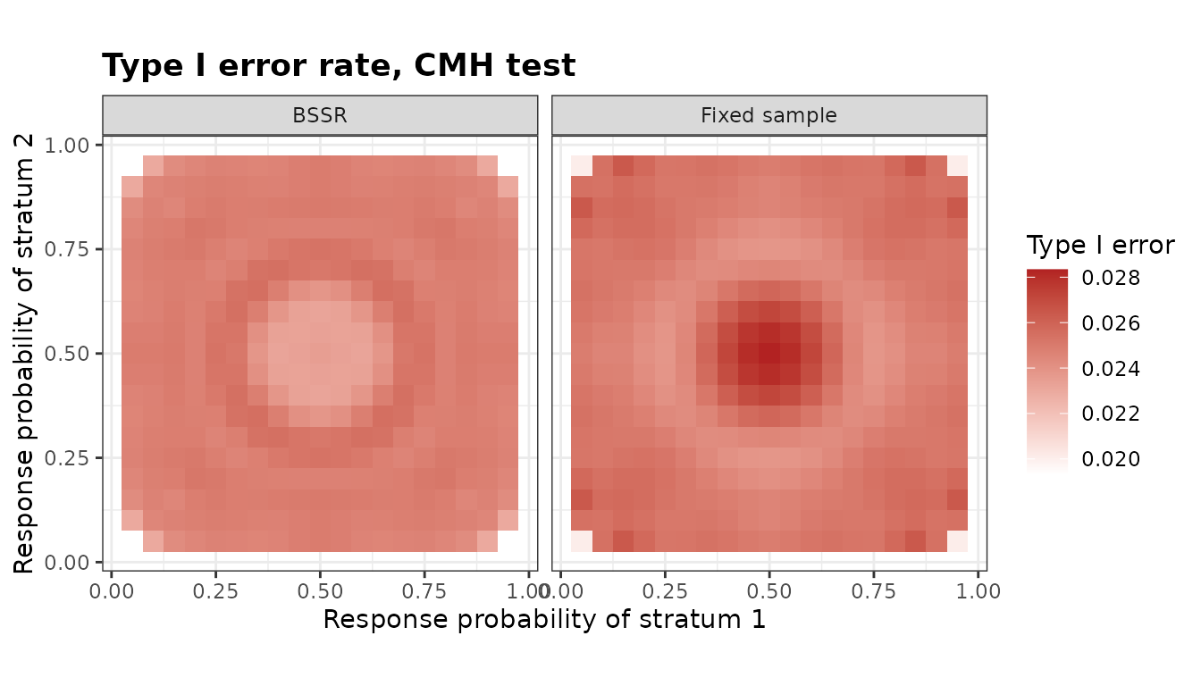

StratAlphaAdjBSSR() lowers the nominal level until the certified largest rate does not exceed alpha.

adj <- StratAlphaAdjBSSR(Delta.A = 2.5, N1 = c(20, 20), N2 = c(20, 20), omega = 0.5,
                         r = 1, alpha = 0.025, tar.power = 0.8, Test = 'CMH',
                         effect = 'OR', ss.method = 'standard', N.max = 160,
                         theta = seq(0.05, 0.95, by = 0.05))
adj
#> Adjusted significance level for blinded sample size re-estimation
#> 
#>   Test            : CMH
#>   Alternative     : greater
#>   Adjusted part   : final analysis only
#>   Maximum         : certified over (theta.S1, theta.S2) in [0.05, 0.95] x [0.05, 0.95]
#>   Target level    : 0.025
#> 
#>        Design   max.TIE alpha.adj max.TIE.adj
#>          BSSR 0.0255490 0.0245872   0.0248681
#>  Fixed sample 0.0283368 0.0228356   0.0246744

StratCondRejectBSSR() gives, under the null hypothesis, the probability of rejection given the pooled numbers of responders of the strata at the interim analysis and in the second stage. These probabilities do not depend on $(\theta_1, \theta_2)$ , and averaging them over the second stage gives the type I error rate given the interim outcome. Below they are evaluated at the point of the largest rate found above.

crp <- StratCondRejectBSSR(Delta.A = 2.5, N1 = c(20, 20), N2 = c(20, 20), omega = 0.5,
                           r = 1, alpha = 0.025, tar.power = 0.8, Test = 'CMH',
                           effect = 'OR', ss.method = 'standard', N.max = 160,
                           theta = cbind(mx$theta.S1[1], mx$theta.S2[1]))
crp
#> Conditional rejection probabilities of blinded sample size re-estimation
#> for a stratified design, under equal response probabilities in every stratum
#> 
#>   Test             : CMH
#>   Alternative      : greater
#>   Planned sizes    : (20, 20) and (20, 20)
#>   Interim sizes    : (10, 10) and (10, 10)
#>   Assumed effect   : 2.5 (OR)
#>   Nominal level    : 0.025
#>   Interim outcomes : 441 pairs (s1, s2)
#>   Above the level  : 267496 outcomes for CRP, 762792 for CRP.total
#> 
#> Largest conditional rejection probability
#>   Quantity   value s1 s2 w1 w2
#>        CRP 0.06250  1  1  1  1
#>  CRP.total 0.06093  1  0  1  2
#> 
#> Type I error rate over 1 point: largest 0.02555 at theta = (0.340135, 0.340135)
by.s <- attr(crp, 'by.s')
head(by.s[order(-by.s$contribution), ], 5)
#>      theta.S1  theta.S2 s1 s2     prob.s      TIE.s contribution
#> 155 0.3401352 0.3401352  7  7 0.03371154 0.02640780 0.0008902478
#> 134 0.3401352 0.3401352  7  6 0.03270032 0.02633070 0.0008610225
#> 154 0.3401352 0.3401352  6  7 0.03270032 0.02633070 0.0008610225
#> 133 0.3401352 0.3401352  6  6 0.03171943 0.02617832 0.0008303614
#> 176 0.3401352 0.3401352  7  8 0.02823765 0.02625803 0.0007414652

The contributions of the interim outcomes sum to 0.02555, the largest type I error rate found above.

Analyses that ignore the strata

'Unstrat-Chisq' is Pearson’s chi-squared test of the table of totals, with $\sum_j N_{1j}$ and $\sum_j N_{2j}$ patients and $\sum_j z_j$ responders, which is the comparison of two proportions with the pooled variance; 'Unstrat-Chisq-cc' adds the continuity correction, and 'Unstrat-Fisher' is Fisher’s exact test of that table. Their critical values depend on $z$ only through $\sum_j z_j$ , but their power and type I error rate are computed with the response probabilities of each stratum. An unstratified test controls the level when the strata are distributed alike in the two groups, and its level can be distorted otherwise (Nam, 1992; Jung, 2014). In the next design group 1 holds a third of the first stratum, whose patients respond rarely, and three quarters of the second.

th <- rbind(c(0.2, 0.6), c(0.4, 0.4))
lev <- sapply(c('CMH', 'Strat-Fisher', 'Unstrat-Chisq', 'Unstrat-Fisher'), function(Test) {
  StratPower(th, th, N1 = c(20, 60), N2 = c(40, 20), alpha = 0.025, Test = Test)$Power
})
rownames(lev) <- c('theta = (0.2, 0.6)', 'theta = (0.4, 0.4)')
round(lev, 4)
#>                       CMH Strat-Fisher Unstrat-Chisq Unstrat-Fisher
#> theta = (0.2, 0.6) 0.0264       0.0157        0.5090         0.4348
#> theta = (0.4, 0.4) 0.0247       0.0160        0.0247         0.0166

With the response probabilities 0.2 and 0.6 in the two strata, the one-sided type I error rate of the unstratified chi-squared test is 0.509 instead of 0.025, because the table of totals compares groups made of different mixtures of the strata. When the strata respond alike, the rate is 0.0247.

The re-estimation can ignore the strata as well: with ss.strata = 'pooled' the sample size is re-estimated from the proportion of responders among all the interim patients, used for every stratum, so the final sizes depend only on the total number of interim responders. The final analysis is still the test given by Test.

res.pooled <- StratPowerBSSR(p = rbind(pooled, pooled + 0.1), Delta.A = 2.5,
                             Delta.T = 2.5, N1 = plan$N1, N2 = plan$N2, omega = 0.5, r = 1,
                             alpha = 0.025, tar.power = 0.8, Test = 'CMH', effect = 'OR',
                             ss.method = 'standard', N.max = 2 * plan$N,
                             ss.strata = 'pooled')
rbind(stratified = res$E.N, pooled = res.pooled$E.N)
#>                [,1]     [,2]
#> stratified 166.4284 175.7539
#> pooled     157.1181 165.4599

The rows give the expected final totals of the two estimates in the two scenarios of the previous section.

Random stratum and group sizes

When the patients are enrolled one at a time, the size of each stratum is known only at the end of the enrolment, and the sizes of the groups within a stratum depend on the randomization. With two strata, StratPower() describes such a design by its total N, the fractions of the strata frac and the allocation ratio r, StratSampleSize() searches the total for the same description, and alloc chooses how the sizes are drawn. With alloc = 'stratum' the size of stratum 1 is binomial with the probability frac[1], and within each stratum the groups are allocated by permuted blocks of size block, as in stratified block randomization. With 'group' the size of stratum 1 is fixed at floor(N * frac[1]), and each patient is in group 1 with the probability $r / (1 + r)$ (Jung, 2014, Section 3.2, where the size of stratum 1 is the round-off of N * frac[1]; the integer part used here reproduces all but one of the sample sizes of the column ‘n fixed’ of Table 4 of the article). With 'both' the stratum sizes are binomial as well (Jung, 2014, Section 3.1). The power is the sum over the stratum and group sizes of their probability times the power of the fixed design they give. Sizes whose probability is below $10^{-14}$ are left out, and the attribute skipped gives their total probability, a bound on the error of the power.

alloc.power <- function(alloc) {
  StratPower(p1, p2, alpha = 0.025, Test = 'CMH', alloc = alloc, N = 80,
             frac = c(0.5, 0.5))$Power
}
pw <- c(fixed = StratPower(p1, p2, N1 = c(20, 20), N2 = c(20, 20), alpha = 0.025,
                           Test = 'CMH')$Power,
        stratum = alloc.power('stratum'), group = alloc.power('group'))
round(pw, 4)
#>   fixed stratum   group 
#>  0.5171  0.5183  0.4979

For the design of the section on the type I error rate, with 20 patients in each group and stratum and 80 in all, the power of the CMH test with the planning probabilities is 0.5171 with fixed group sizes, 0.5183 with permuted blocks in random strata and 0.4979 with random groups in fixed strata. Permuted blocks keep the power within 0.002 of that with fixed sizes, while binomial group sizes, which vary around the planned sizes, lower it by about 0.02. The number of configurations of the sizes grows most quickly with 'both', whose power takes far longer to compute than with the other models.

StratPowerBSSR(), StratTypeIErrorBSSR(), StratAlphaAdjBSSR() and StratBSSR() take alloc and block as well. With two strata the interim analysis has the first patients enrolled, as many as the interim total of the design, and the final analysis the first N patients, where N is the total re-estimated from the interim data with the fractions of the strata among the interim patients (ss.frac = 'observed', the default) or with those of the plan ('planned'). Given an allocation sequence, that is the strata and the groups of the patients in the order of enrolment, the design has fixed group sizes and is computed exactly. The power and the type I error rate are averaged over nseq sequences drawn with the random numbers of R, and se.BSSR is the Monte Carlo standard error of the average. The power of the fixed design with the same allocation is exact.

bssr.small <- function(...) {
  StratPowerBSSR(p = rbind(pooled, pooled + 0.1), Delta.A = 2.5, Delta.T = 2.5,
                 N1 = c(20, 20), N2 = c(20, 20), omega = 0.5, r = 1, alpha = 0.025,
                 tar.power = 0.8, Test = 'CMH', effect = 'OR', ss.method = 'standard',
                 N.max = 160, ...)
}
res.small <- bssr.small()
set.seed(2)
res.alloc <- bssr.small(alloc = 'stratum', nseq = 20)
res.small[, c('power.BSSR', 'power.TRAD', 'E.N')]
#>   power.BSSR power.TRAD      E.N
#> 1  0.7946358  0.5171358 159.2986
#> 2  0.7819219  0.4832641 159.7109
res.alloc[, c('power.BSSR', 'se.BSSR', 'power.TRAD', 'E.N')]
#>   power.BSSR      se.BSSR power.TRAD      E.N
#> 1  0.7954675 0.0004363258  0.5182658 159.3638
#> 2  0.7798800 0.0008324083  0.4879723 159.7567

With fixed group sizes the re-estimation raises the power from 0.5171, that of the fixed design with 80 patients, to 0.7946 in the first scenario, with an expected total of 159.3 close to the bound of 160. With permuted blocks in random strata and 20 sequences, the power of the re-estimation design is 0.7955 and 0.7799 in the two scenarios, with the standard errors 0.00044 and 0.00083, against 0.7946 and 0.7819 with fixed group sizes, and the expected totals are 159.4 and 159.8, against 159.3 and 159.7. For this design the random sizes change the power of the re-estimation design by less than 0.01 and its expected total by less than one patient. The default nseq = 100 divides the standard errors by about 2.2.

Several designs

StratGridBSSR() evaluates several re-estimation designs over common scenarios, as BinaryGridBSSR() does for two groups (see vignette('bbssr-design-grid')). Each row of a data frame is a design, whose columns are arguments of StratPowerBSSR(); an argument with one value per stratum is given by the columns with the suffixes .S1, .S2, and so on, or as a vector shared by all designs. Below, two tests and two timings of the interim analysis are compared for the design of the section on the type I error rate, with the pooled response probability of stratum 2 varying between the scenarios.

design <- expand.grid(Test = c('CMH', 'Cochran'), omega = c(0.3, 0.5),
                      stringsAsFactors = FALSE)
q <- cbind(0.4, c(0.5, 0.6, 0.7))
grid <- StratGridBSSR(design, p = q, Delta.A = 2.5, effect = 'OR', N1 = c(20, 20),
                      N2 = c(20, 20), r = 1, alpha = 0.025, tar.power = 0.8,
                      ss.method = 'standard', N.max = 160)
summary(grid)[, c('Test', 'omega', 'power.BSSR.min', 'power.BSSR.max', 'E.N.max')]
#>      Test omega power.BSSR.min power.BSSR.max  E.N.max
#> 1     CMH   0.3      0.7761882      0.8008585 159.7052
#> 2 Cochran   0.3      0.7804618      0.8036203 159.7052
#> 3     CMH   0.5      0.7764089      0.7998569 159.7730
#> 4 Cochran   0.5      0.7807565      0.8027385 159.7730

The summary gives the range of the power of each design over the scenarios and its largest expected total sample size. The plot draws the power against the probability that varies between the scenarios, here that of stratum 2, with the fixed design as dashed lines.

plot(grid, colour.by = 'Test', facet.by = 'omega')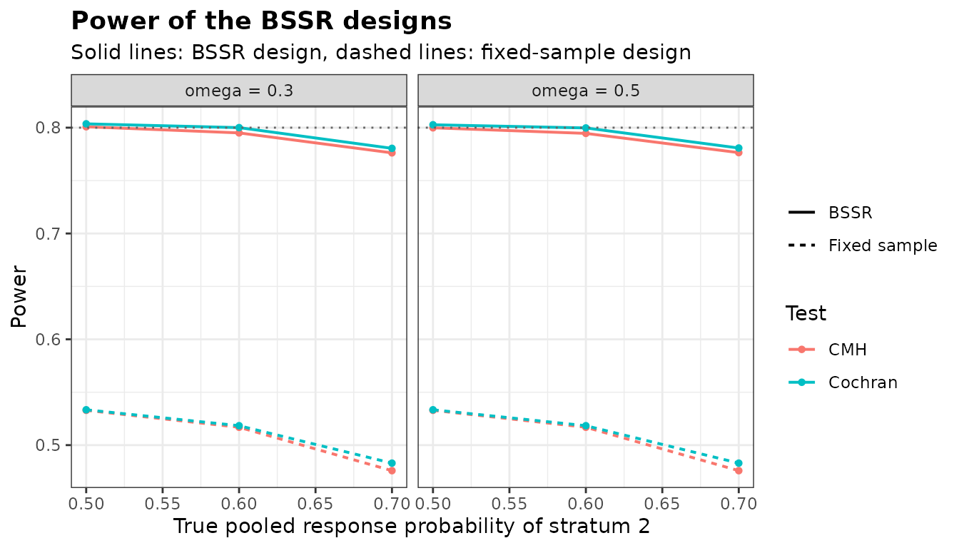

Three or more strata

With three or more strata the number of interim outcomes grows as a product over the strata, and StratPowerBSSR() and StratTypeIErrorBSSR() estimate the rates of the re-estimation design by simulation, with the random numbers of R and a Monte Carlo standard error. With fixed group sizes the rates of the fixed design remain exact. With alloc = 'stratum' or 'both' the strata and the groups of the patients are simulated with the responses, in the fixed design as well, whose standard error is se.TRAD. The model 'group' needs two strata.

set.seed(1)
q2 <- c(0.2, 0.35, 0.5)
q1 <- q2 * 2.5 / (1 - q2 + q2 * 2.5)
plan3 <- StratSampleSize(q1, q2, frac = c(0.3, 0.3, 0.4), alpha = 0.025,
                         tar.power = 0.8, Test = 'CMH', method = 'standard')
res3 <- StratPowerBSSR(p = (q1 + q2) / 2, Delta.A = 2.5, Delta.T = 2.5, N1 = plan3$N1,
                       N2 = plan3$N2, omega = 0.5, r = 1, alpha = 0.025, tar.power = 0.8,
                       Test = 'CMH', effect = 'OR', ss.method = 'standard',
                       N.max = 2 * plan3$N, nsim = 2e4)
res3[, c('power.BSSR', 'se.BSSR', 'power.TRAD', 'E.N')]
#>   power.BSSR     se.BSSR power.TRAD      E.N
#> 1    0.82235 0.002702688  0.8033501 175.9536

References

Jung, S. H. (2014). Stratified Fisher’s exact test and its sample size calculation. Biometrical Journal, 56, 129-140.

Nam, J. (1992). Sample size determination for case-control studies and the comparison of stratified and unstratified analyses. Biometrics, 48, 389-395.

Woolson, R. F., Bean, J. A. and Rojas, P. B. (1986). Sample size for case-control studies using Cochran’s statistic. Biometrics, 42, 927-932.

Gosuke Homma

2026-10-28