Type I Error Rate of a Re-estimation Design

library(bbssr)

The type I error rate of a re-estimation design

With blinded sample size re-estimation the final sample size depends on the pooled number of interim responders, whose distribution depends on the common response probability $\theta$ . The type I error rate of a re-estimation design is computed for the design itself, by summing the rejection probability over the interim outcomes and the outcomes of the second stage.

Under the null hypothesis $p_{1} = p_{2} = \theta$ . Let $n_{11}$ and $n_{12}$ be the interim sample sizes of the two groups, $s$ the pooled number of interim responders, $n_{21}(s)$ and $n_{22}(s)$ the second-stage sample sizes reached from $s$ , and $\mathcal{R}_{s}$ the rejection region at the final sample size reached from $s$ . The type I error rate is $\mathrm{TIE}(\theta) = \sum_{s = 0}^{n_{11} + n_{12}} \Pr_{\theta}(S = s) \, \Pr_{\theta}\bigl((X_{1}, X_{2}) \in \mathcal{R}_{s} \mid S = s\bigr) ,$ a polynomial in $\theta$ that the package evaluates exactly.

The rate over the nuisance parameter

BinaryTypeIErrorBSSR() evaluates the type I error rate of a re-estimation design and of the fixed-sample design with the initial sample size over a grid of $\theta$ , by default seq(0, 1, by = 0.005). The largest value is not read off the grid. With the default maximize = 'certified' the function finds the largest value over the whole interval spanned by the grid, here $[0, 1]$ , together with an upper bound that the rate does not exceed anywhere in that interval. The bbssr-statistical-methods vignette describes the method. The design below has an assumed difference of 0.3, an initial sample size of 39 per group, an interim analysis after 20 per group, re-estimation by formula (21.3) of Kieser (2020) and the chi-squared test.

design <- list(Delta.A = 0.3, N1 = 39, N2 = 39, n.interim = c(20, 20), r = 1,
               alpha = 0.025, tar.power = 0.8, Test = 'Chisq', ss.method = 'standard')
tie <- do.call(BinaryTypeIErrorBSSR, design)
tie
#> Type I error rate of blinded sample size re-estimation for a binary endpoint
#> 
#>   Test            : Chisq
#>   Alternative     : greater
#>   Initial size    : N1 = 39, N2 = 39
#>   Interim size    : n1 = 20, n2 = 20
#>   Assumed effect  : 0.3 (RD)
#>   Nominal level   : 0.025
#>   Grid            : 201 values of theta in [0, 1]
#>   Maximum         : certified over theta in [0, 1]
#> 
#> Largest type I error rate
#>        Design     theta     TIE
#>          BSSR 0.4376830 0.02729
#>  Fixed sample 0.0935669 0.02938
attr(tie, 'max')
#>   Design      theta        TIE      bound
#> 1   BSSR 0.43768311 0.02728643 0.02728643
#> 2   TRAD 0.09356689 0.02937611 0.02937611
plot(tie)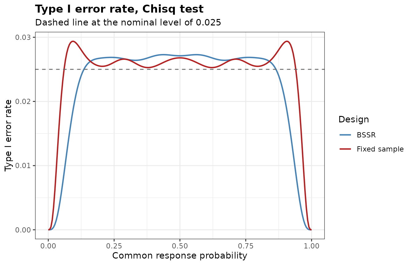

The largest type I error rate is 0.02729 at $\theta =$ 0.4377 for the re-estimation design and 0.02938 at $\theta =$ 0.09357 for the fixed-sample design. The column bound of the attribute max exceeds these values by at most $10^{-12}$ , so the largest rates are known to that accuracy whatever the spacing of the grid. The chi-squared test is not exact, so the fixed-sample design can already exceed the nominal level, and the re-estimation changes the rate again.

Exact tests in the final analysis

The same design with an exact test in the final analysis gives the following largest rates.

exact.max <- do.call(rbind, lapply(c('Fisher', 'Boschloo'), function(tst) {
  m <- attr(do.call(BinaryTypeIErrorBSSR, modifyList(design, list(Test = tst))), 'max')
  data.frame(Test = tst, Design = m$Design, theta = signif(m$theta, 4),
             TIE = signif(m$TIE, 4))
}))
exact.max
#>       Test Design  theta     TIE
#> 1   Fisher   BSSR 0.4741 0.01573
#> 2   Fisher   TRAD 0.5000 0.01540
#> 3 Boschloo   BSSR 0.3726 0.02312
#> 4 Boschloo   TRAD 0.4543 0.02477

For this rule the largest rate of the re-estimation design is 0.01573 with Fisher’s exact test and 0.02312 with the Boschloo test, against the nominal 0.025.

The adjusted significance level

When the rate exceeds the nominal level, BinaryAlphaAdjBSSR() lowers the nominal level until the largest type I error rate does not exceed the target level, following Kieser and Friede (2000) and Friede and Kieser (2004). With adjust = 'test' (the default) the adjusted level is applied to the final analysis only. The re-estimated sample sizes then do not depend on the level, the largest rate is a non-decreasing step function of it, and the level is found by bisection. Every level between the largest p-value that is rejected and the smallest p-value that is not gives the same rejection regions, and the reported level is the largest value with at most six significant digits in that range, so it can be used as printed.

Both searches below use the grid theta.grid from 0.01 to 0.99 in steps of 0.01, which is coarser than the default to keep them short. The grid serves the search: a level is assessed on the grid, and with the default maximize = 'certified' the level found is accepted only if the upper bound of the type I error rate over the whole interval $[0.01, 0.99]$ does not exceed the target level. The columns max.TIE.bound and max.TIE.adj.bound of the result hold the bounds at the nominal and at the adjusted level.

theta.grid <- seq(0.01, 0.99, by = 0.01)
adj <- do.call(BinaryAlphaAdjBSSR, c(design, list(theta = theta.grid)))
adj
#> Adjusted significance level for blinded sample size re-estimation
#> 
#>   Test            : Chisq
#>   Alternative     : greater
#>   Adjusted part   : final analysis only
#>   Maximum         : certified over theta in [0.01, 0.99]
#>   Target level    : 0.025
#> 
#>        Design   max.TIE alpha.adj max.TIE.adj
#>          BSSR 0.0272864 0.0204375   0.0237418
#>  Fixed sample 0.0293761 0.0207700   0.0247660

With adjust = 'both' the adjusted level is used in the re-estimation as well. The re-estimated sample sizes then change with the level, the rate need not be monotone in it, and the level is lowered in steps of step until the rate is controlled. The result is the first level on this grid of steps at which the rate is controlled. The levels that control the rate need not form an interval, so the result can change with the step. The published values of Friede and Kieser (2004, Section 5) and Kieser (2020, Example 21.1) are reproduced only when the re-estimation also uses the adjusted level, as the script reproduce-published.R shows (see the bbssr-validation vignette). The search below uses a step of 0.00005, coarser than the default, to keep it short.

adj.both <- do.call(BinaryAlphaAdjBSSR,
                    c(design, list(adjust = 'both', step = 5e-5, theta = theta.grid)))
adj.both
#> Adjusted significance level for blinded sample size re-estimation
#> 
#>   Test            : Chisq
#>   Alternative     : greater
#>   Adjusted part   : final analysis and re-estimation
#>   Maximum         : certified over theta in [0.01, 0.99]
#>   Target level    : 0.025
#> 
#>        Design   max.TIE alpha.adj max.TIE.adj
#>          BSSR 0.0272864   0.02110   0.0246043
#>  Fixed sample 0.0293761   0.02077   0.0247660

The adjusted level of the re-estimation design is 0.0204375 when it applies to the final analysis only and 0.0211 when it also applies to the re-estimation. At these levels the upper bounds of the type I error rate over $[0.01, 0.99]$ are 0.02374 and 0.0246. The power at the adjusted level follows from BinaryPowerBSSR() with alpha set to the adjusted level. The re-estimation keeps the target level through ss.alpha when the level was adjusted with adjust = 'test'.

adjusted <- modifyList(design, list(alpha = adj$alpha.adj[1], ss.alpha = 0.025))
power.adj <- do.call(BinaryPowerBSSR,
                     c(adjusted, list(p = c(0.3, 0.4, 0.5), Delta.T = 0.3)))
power.nominal <- do.call(BinaryPowerBSSR,
                         c(design, list(p = c(0.3, 0.4, 0.5), Delta.T = 0.3)))
data.frame(p = power.adj$p, power.nominal = round(power.nominal$power.BSSR, 4),
           power.adjusted = round(power.adj$power.BSSR, 4))
#>     p power.nominal power.adjusted
#> 1 0.3        0.7984         0.7730
#> 2 0.4        0.8031         0.7685
#> 3 0.5        0.8037         0.7646

Control within a confidence interval

The largest type I error rate over the whole range of the nuisance parameter can occur at values that the data of the completed trial make implausible. Kieser (2020, Section 22.1.3) describes another way to control the type I error rate. A value $0 < \gamma < \alpha$ is fixed in advance, the $(1 - \gamma)$ confidence interval for the nuisance parameter is computed from the data of the completed trial, and the final analysis uses a level at which the largest type I error rate over this interval does not exceed $\alpha - \gamma$ . The type I error rate is then controlled at $\alpha$ . BinaryAlphaAdjBSSR() finds this level when theta spans the interval and alpha is set to $\alpha - \gamma$ . The interval is known only at the end of the trial, so the re-estimation keeps the nominal level, through adjust = 'test' and ss.alpha.

Example 23.1 of Kieser (2020) applies the approach to the FreezeAF trial, a non-inferiority trial with the margin 0.15 and the test of Farrington and Manning (1990), equal assumed rates of 0.78, an initial sample size of 122 per group and a pilot of 100 patients. The rate is evaluated on the boundary of the null hypothesis against the pooled response probability, as described in the bbssr-non-inferiority vignette, on the grid of the book with steps of 0.005. For control over the whole range, the book applies the adjusted level to the re-estimation as well, which is adjust = 'both'. A step of 0.0001 keeps the search short.

freeze <- list(Delta.A = 0, N1 = 122, N2 = 122, n.interim = c(50, 50), r = 1,
               alpha = 0.025, tar.power = 0.8, Test = 'Farrington-Manning',
               ss.method = 'standard', margin = 0.15)
adj.whole <- do.call(BinaryAlphaAdjBSSR,
                     c(freeze, list(theta = seq(0.075, 0.925, by = 0.005),
                                    maximize = 'grid', adjust = 'both', step = 1e-4)))
adj.whole[1, c('Design', 'max.TIE', 'alpha.adj', 'max.TIE.adj', 'theta.adj')]
#>   Design    max.TIE alpha.adj max.TIE.adj theta.adj
#> 1   BSSR 0.02644929    0.0241  0.02492749      0.85

The trial observed 210 responders among 291 patients. With $\gamma = 0.0001$ the interval is the 99.99 per cent Clopper-Pearson interval, which binom.test() returns. The book calls it a 95 per cent interval, but the interval it gives is the 99.99 per cent interval. The code below computes the largest type I error rate within the interval at the nominal level and the adjusted level.

gamma <- 1e-4
ci <- binom.test(210, 291, conf.level = 1 - gamma)$conf.int
ci.grid <- seq(ci[1], ci[2], length.out = 42)
tie.ci <- do.call(BinaryTypeIErrorBSSR,
                  c(freeze, list(theta = ci.grid, maximize = 'grid')))
adj.ci <- do.call(BinaryAlphaAdjBSSR,
                  c(modifyList(freeze, list(alpha = 0.025 - gamma)),
                    list(ss.alpha = 0.025, theta = ci.grid, maximize = 'grid')))
adj.ci[1, c('Design', 'alpha', 'alpha.adj', 'max.TIE.adj', 'theta.adj')]
#>   Design  alpha alpha.adj max.TIE.adj theta.adj
#> 1   BSSR 0.0249 0.0241286  0.02489991 0.7662331

Within the interval $[0.611, 0.816]$ the largest rate of the re-estimation design is 0.026, only slightly below the largest rate 0.0264 over the whole range, as the book notes. The adjusted level that keeps the rate within the interval at or below $\alpha - \gamma = 0.0249$ is 0.0241, and the level that controls the rate over the whole range is 0.0241. The book reports 0.0241 for both, and reproduce-published.R reproduces these values with a step of $10^{-5}$ (see the bbssr-validation vignette).

Conditional rejection probabilities

BinaryCondRejectBSSR() takes the calculation apart. Given the pooled number $s$ of interim responders and the pooled number $s_{2}$ of second-stage responders, the number of responders of group 1 in each stage is hypergeometric under the null hypothesis, and the two stages are independent. The rejection probability given $s$ and $s_{2}$ , $\mathrm{CRP}(s, s_{2}) = \sum_{x_{11}} \sum_{x_{21}} h_{1}(x_{11} \mid s) \, h_{2}(x_{21} \mid s_{2}) \, \mathbf{1}\bigl\{(x_{11} + x_{21}, \, s + s_{2} - x_{11} - x_{21}) \in \mathcal{R}_{s}\bigr\} ,$ where $h_{1}$ and $h_{2}$ are the hypergeometric probabilities of the two stages, does not depend on $\theta$ . The type I error rate is its average over the binomial distributions of $s$ and $s_{2}$ , $\mathrm{TIE}(\theta) = \sum_{s} \sum_{s_{2}} b(s; n_{11} + n_{12}, \theta) \, b\bigl(s_{2}; n_{21}(s) + n_{22}(s), \theta\bigr) \, \mathrm{CRP}(s, s_{2}) ,$ where $b$ is the binomial probability. The column CRP.total is the rejection probability given only the total $s + s_{2}$ , with the responder count of group 1 treated as one hypergeometric count among all final patients.

crp <- BinaryCondRejectBSSR(
  Delta.A = 0.3, N1 = 12, N2 = 12, n.interim = c(6, 6), r = 1, alpha = 0.025,
  tar.power = 0.8, Test = 'Chisq', ss.method = 'standard', theta = c(0.3, 0.5)
)
crp
#> Conditional rejection probabilities of blinded sample size re-estimation
#> for a binary endpoint, under equal response probabilities
#> 
#>   Test            : Chisq
#>   Alternative     : greater
#>   Initial size    : N1 = 12, N2 = 12
#>   Interim size    : n1 = 6, n2 = 6
#>   Assumed effect  : 0.3 (RD)
#>   Nominal level   : 0.025
#>   Outcomes        : 567 pairs (s, s2)
#>   Above the level : 198 for CRP, 264 for CRP.total
#> 
#> Largest conditional rejection probability
#>   Quantity   value s s2 N1 N2
#>        CRP 0.05519 2  2 24 24
#>  CRP.total 0.05753 4  0 38 38
#> 
#> Type I error rate over 2 values of theta: largest 0.02762 at theta = 0.5
plot(crp)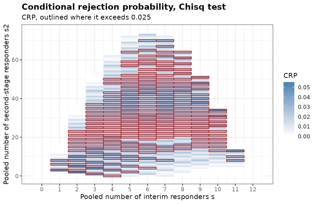

The decomposition by $s$ is returned when theta is given.

by.s <- attr(crp, 'by.s')
head(by.s)
#>   theta s N1 N2     prob.s      TIE.s contribution
#> 1   0.3 0  6  6 0.01384129 0.00000000  0.000000000
#> 2   0.3 1 14 14 0.07118376 0.02078361  0.001479455
#> 3   0.3 2 24 24 0.16779030 0.02603899  0.004369090
#> 4   0.3 3 32 32 0.23970043 0.02648734  0.006349026
#> 5   0.3 4 38 38 0.23113970 0.02684226  0.006204313
#> 6   0.3 5 42 42 0.15849579 0.02550149  0.004041879
attr(crp, 'TIE')
#>   theta        TIE
#> 1   0.3 0.02537642
#> 2   0.5 0.02761990
plot(crp, what = 'by.s')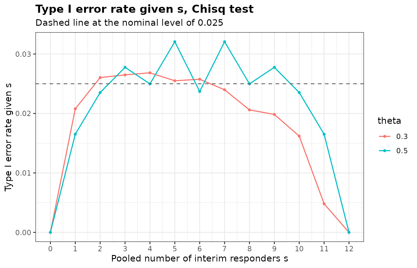

TIE.s is the type I error rate given $s$ , and contribution is its product with the probability prob.s of $s$ . The contributions add up to the type I error rate at each value of theta, which is 0.02538 and 0.02762 here.

Non-inferiority

With a non-inferiority margin, BinaryTypeIErrorBSSR() and BinaryAlphaAdjBSSR() evaluate the rate on the boundary of the null hypothesis, parametrized by the pooled response probability, see the bbssr-non-inferiority vignette. BinaryCondRejectBSSR() covers tests of superiority only, since on the boundary of a non-inferiority hypothesis the two response probabilities differ and the conditional distributions of the responder counts depend on them.

References

Farrington, C. P. and Manning, G. (1990). Test statistics and sample size formulae for comparative binomial trials with null hypothesis of non-zero risk difference or non-unity relative risk. Statistics in Medicine, 9, 1447-1454.

Friede, T. and Kieser, M. (2004). Sample size recalculation for binary data in internal pilot study designs. Pharmaceutical Statistics, 3, 269-279.

Kieser, M. (2020). Methods and Applications of Sample Size Calculation and Recalculation in Clinical Trials. Springer.

Kieser, M. and Friede, T. (2000). Re-calculating the sample size in internal pilot study designs with control of the type I error rate. Statistics in Medicine, 19, 901-911.

Gosuke Homma

2026-10-28