
Non-inferiority and Equivalence Trials
Gosuke Homma
2026-10-28
Source:vignettes/bbssr-non-inferiority.Rmd
bbssr-non-inferiority.RmdHypotheses and margin
Let group 1 receive the experimental treatment and group 2 the
control. A non-inferiority trial with a margin
on the scale of the risk difference tests
which corresponds to
alternative = 'greater' and margin = delta.
With alternative = 'less' the null hypothesis is
,
which suits an endpoint for which a lower response probability is
better. A negative margin tests superiority by more than its absolute
value. A margin other than 0 requires one of the two tests below and a
one-sided alternative. The last section covers a margin on the scale of
the risk ratio, margin.scale = 'RR'.
The two tests
Both tests refer
to the standard normal distribution and
reject
when
.
The test of Blackwelder (1982), Test = 'Blackwelder', uses
the standard error at the observed proportions,
The test of Farrington and Manning
(1990), Test = 'Farrington-Manning', uses the same
expression at the maximum likelihood estimates
and
under the restriction
.
With
the Farrington-Manning test is the chi-squared test and the Blackwelder
test is the Wald test.
The two tests are asymptotic, but the package computes their rejection regions, power and sample sizes exactly, as for the other tests.
rr.bw <- BinaryRR(N1 = 60, N2 = 60, alpha = 0.025, Test = 'Blackwelder', margin = 0.1)
rr.fm <- BinaryRR(N1 = 60, N2 = 60, alpha = 0.025, Test = 'Farrington-Manning',
                  margin = 0.1)
c(Blackwelder = sum(rr.bw), Farrington.Manning = sum(rr.fm))
#>        Blackwelder Farrington.Manning
#>               1714               1698
plot(rr.fm)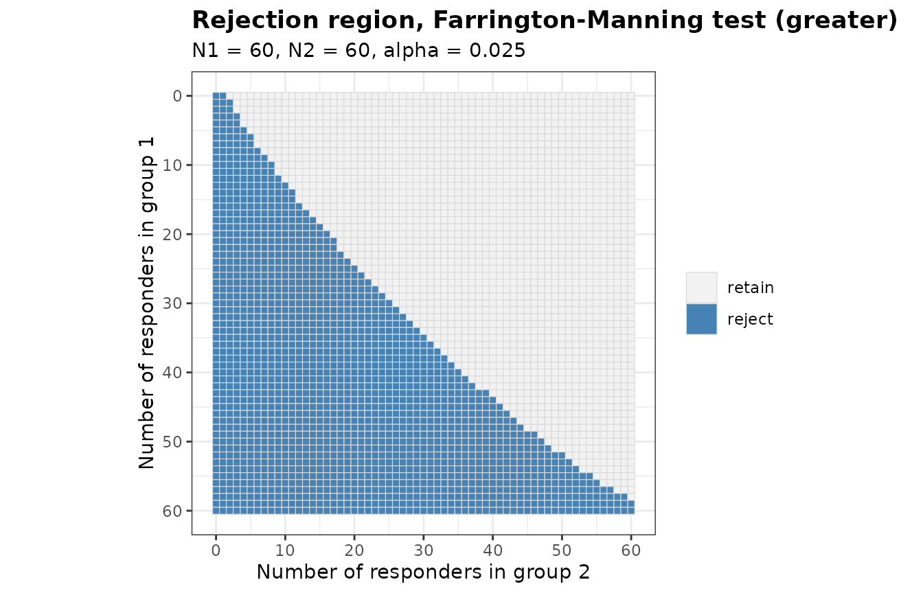
The size of a test of non-inferiority is its largest rejection probability on the boundary of the null hypothesis. The function below evaluates it over a fine grid of .
boundary_size <- function(RR, margin) {
  N1 <- attr(RR, 'N1')
  N2 <- attr(RR, 'N2')
  m <- matrix(as.vector(RR), N1 + 1L, N2 + 1L)
  p2 <- seq(margin + 0.001, 0.999, by = 0.001)
  size <- vapply(p2, function(q) {
    sum(outer(dbinom(0:N1, N1, q - margin), dbinom(0:N2, N2, q)) * m)
  }, numeric(1))
  data.frame(p2 = p2[which.max(size)], size = max(size))
}
sizes <- cbind(Test = c('Blackwelder', 'Farrington-Manning'),
               rbind(boundary_size(rr.bw, 0.1), boundary_size(rr.fm, 0.1)))
sizes
#>                 Test    p2       size
#> 1        Blackwelder 0.993 0.06067597
#> 2 Farrington-Manning 0.550 0.02730085
The nominal level is 0.025. With 60 patients per group the size is 0.0607 for the Blackwelder test, attained at 0.993, and 0.0273 for the Farrington-Manning test. The size of an asymptotic test at a given sample size can lie on either side of the nominal level, so it is worth computing for the sample sizes of a design.
Sample size
With a margin, BinarySampleSize() replaces the
difference in the normal approximation by its distance
from the boundary of the null hypothesis.
method = 'standard' evaluates the variance in the term of
the significance level at the large sample values of the restricted
estimates, which gives formula (4) of Farrington and Manning (1990).
method = 'alternative.variance' uses the variance under the
alternative in both terms, which gives the formula of Blackwelder
(1982). method = 'exact' steps from the formula of
Farrington and Manning, one patient at a time, to the sample size at
which the exact power of the test first attains the target. Below, both
groups have a response probability of 0.7 and the margin is 0.15.
ni.ss <- expand.grid(method = c('exact', 'standard', 'alternative.variance'),
                     Test = c('Blackwelder', 'Farrington-Manning'),
                     stringsAsFactors = FALSE)
ni.ss$N <- NA
ni.ss$Power <- NA
for (i in seq_len(nrow(ni.ss))) {
  ss <- BinarySampleSize(p1 = 0.7, p2 = 0.7, r = 1, alpha = 0.025, tar.power = 0.8,
                         Test = ni.ss$Test[i], method = ni.ss$method[i], margin = 0.15)
  ni.ss$N[i] <- ss$N
  ni.ss$Power[i] <- round(ss$Power, 4)
}
ni.ss
#>                 method               Test   N  Power
#> 1                exact        Blackwelder 292 0.8009
#> 2             standard        Blackwelder 292 0.8009
#> 3 alternative.variance        Blackwelder 294 0.8024
#> 4                exact Farrington-Manning 290 0.8005
#> 5             standard Farrington-Manning 292 0.8020
#> 6 alternative.variance Farrington-Manning 294 0.8062
Power is the exact power of the test at the sample size
of each row, so the rows of the two formulas show how close the normal
approximation comes to the target for each test.
Blinded sample size re-estimation
Friede, Mitchell and Mueller-Velten (2007) re-estimate the sample
size of a non-inferiority trial from the blinded overall response rate,
which is the pooled response probability of the package. The assumed
difference is usually 0, so both recovered probabilities equal the
blinded pooled response probability, and the sample size is re-estimated
by the formula of Farrington and Manning
(ss.method = 'standard') or of Blackwelder
(ss.method = 'alternative.variance'). The design below is
planned for a pooled response probability of 0.7 and re-estimates the
sample size after half of the patients.
plan <- BinarySampleSize(p1 = 0.7, p2 = 0.7, r = 1, alpha = 0.025, tar.power = 0.8,
                         Test = 'Farrington-Manning', method = 'standard', margin = 0.15)
ni <- BinaryPowerBSSR(
  p = seq(0.4, 0.8, by = 0.1), Delta.A = 0, Delta.T = 0,
  N1 = plan$N1, N2 = plan$N2, omega = 0.5, r = 1, alpha = 0.025, tar.power = 0.8,
  Test = 'Farrington-Manning', ss.method = 'standard', margin = 0.15
)
ni
#> Blinded sample size re-estimation for a binary endpoint
#>
#>   Test            : Farrington-Manning
#>   Alternative     : greater
#>   Design rule     : unrestricted
#>   Initial size    : N1 = 146, N2 = 146
#>   Interim fraction: 0.5, giving n1 = 73 and n2 = 73
#>   Treatment effect: assumed 0, true 0 (risk difference)
#>   Margin          : 0.15
#>   Re-estimation   : normal approximation (standard), group rounding at level 0.025
#>   Alpha           : 0.025, target power 0.8
#>
#>    p  p1  p2 power.BSSR power.TRAD   E.N
#>  0.4 0.4 0.4     0.7978     0.7473 329.0
#>  0.5 0.5 0.5     0.7912     0.7401 342.1
#>  0.6 0.6 0.6     0.7978     0.7473 329.0
#>  0.7 0.7 0.7     0.8015     0.8020 290.8
#>  0.8 0.8 0.8     0.8069     0.8925 228.5
plot(ni)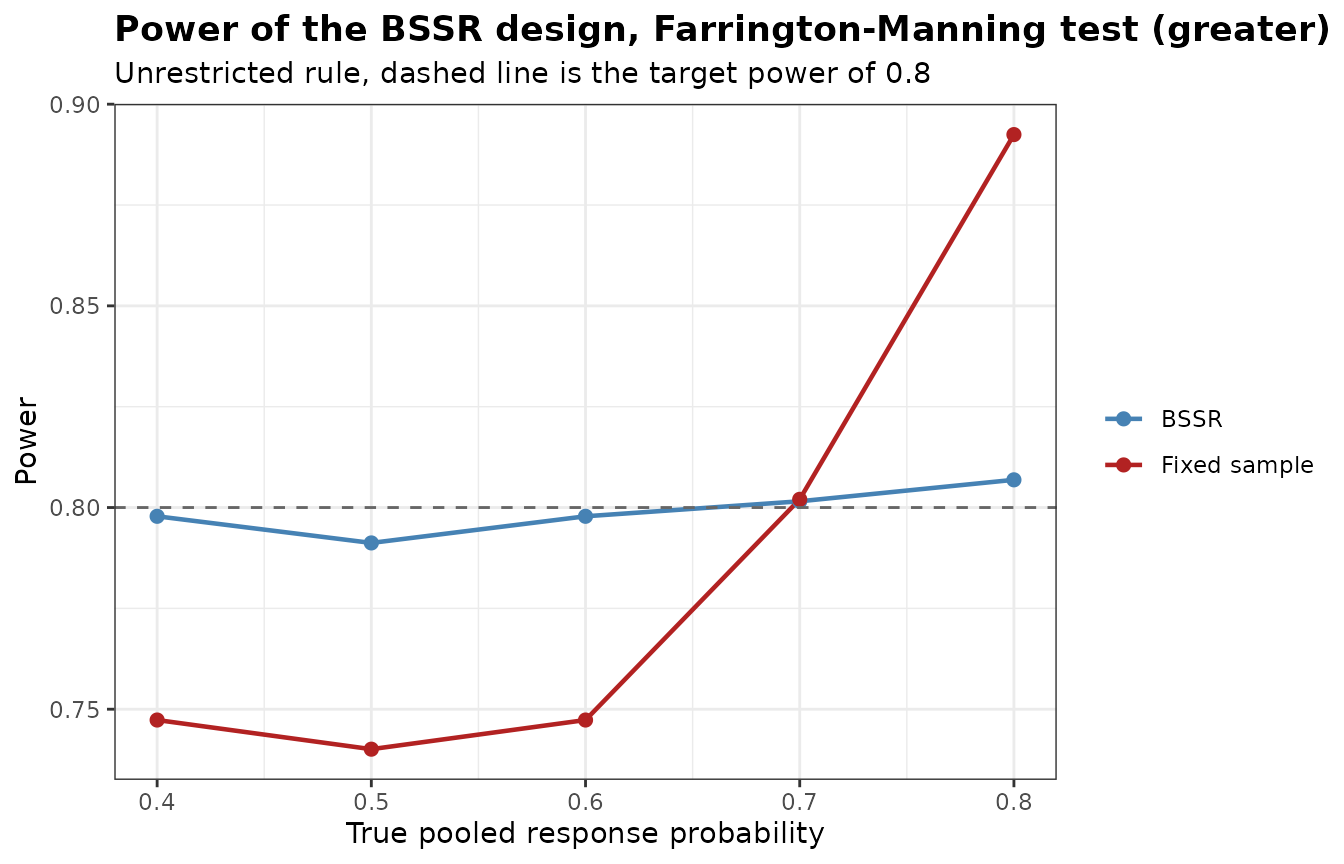
summary(ni)
#>    p1  p2   p      E.N      SD.N N.q25 N.q50 N.q75      P.N.max
#> 1 0.4 0.4 0.4 328.9911 10.868511   322   330   336 4.408925e-02
#> 2 0.5 0.5 0.5 342.0553  3.210567   342   344   344 5.435178e-01
#> 3 0.6 0.6 0.6 328.9911 10.868511   322   330   336 4.408925e-02
#> 4 0.7 0.7 0.7 290.7938 19.451117   278   294   304 8.652446e-06
#> 5 0.8 0.8 0.8 228.4956 24.167543   212   228   244 1.323903e-13
The planned total sample size is 292. The variance of a binary endpoint is largest at one half, so the fixed-sample design loses power when the true pooled response probability lies closer to one half than the planning value, and the re-estimation enlarges the trial in that case. At a pooled response probability of 0.4 the power is 0.798 with re-estimation and 0.747 without.
Type I error rate on the boundary
With a margin, BinaryTypeIErrorBSSR() evaluates the type
I error rate on the boundary of the null hypothesis. The boundary is
parametrized by the pooled response probability theta, and
the values at which a response probability falls outside the unit
interval are dropped.
ni.tie <- BinaryTypeIErrorBSSR(
  Delta.A = 0, N1 = plan$N1, N2 = plan$N2, omega = 0.5, r = 1, alpha = 0.025,
  tar.power = 0.8, Test = 'Farrington-Manning', ss.method = 'standard', margin = 0.15,
  theta = seq(0.1, 0.9, by = 0.01)
)
ni.tie
#> Type I error rate of blinded sample size re-estimation for a binary endpoint
#>
#>   Test            : Farrington-Manning
#>   Alternative     : greater
#>   Initial size    : N1 = 146, N2 = 146
#>   Interim size    : n1 = 73, n2 = 73
#>   Assumed effect  : 0 (RD)
#>   Margin          : 0.15
#>   Nominal level   : 0.025
#>   Grid            : 81 values of theta in [0.1, 0.9]
#>   Maximum         : certified over theta in [0.1, 0.9]
#>
#> Largest type I error rate
#>        Design    theta     TIE
#>          BSSR 0.261652 0.02579
#>  Fixed sample 0.500000 0.02650
plot(ni.tie)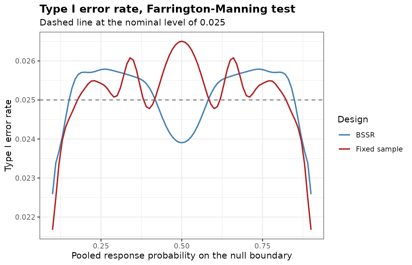
The largest type I error rate is certified over the interval spanned
by theta, here from 0.1 to 0.9. With the default
theta = seq(0, 1, by = 0.005) the interval is the whole
part of the boundary on which both response probabilities lie in the
unit interval, which with an allocation ratio of 1 is theta
from
to
.
The same rejection probabilities follow from
BinaryPowerBSSR() with the true difference on the boundary,
Delta.T = -margin.
on.boundary <- BinaryPowerBSSR(
  p = c(0.5, 0.7), Delta.A = 0, Delta.T = -0.15,
  N1 = plan$N1, N2 = plan$N2, omega = 0.5, r = 1, alpha = 0.025, tar.power = 0.8,
  Test = 'Farrington-Manning', ss.method = 'standard', margin = 0.15
)
rows <- vapply(c(0.5, 0.7), function(t) which.min(abs(ni.tie$theta - t)), integer(1))
max(abs(on.boundary$power.BSSR - ni.tie$TIE.BSSR[rows]))
#> [1] 0
BinaryAlphaAdjBSSR() accepts the margin in the same way
and adjusts the nominal level on the boundary.
Margin on the scale of the risk ratio
With margin.scale = 'RR' the margin is a ratio
,
and alternative = 'greater' tests
With alternative = 'less'
the null hypothesis is
,
as in the second example of Farrington and Manning (1990), where the
relative risk of pertussis among recipients of an acellular vaccine
compared with those of a whole cell vaccine is to be shown to be below
1.5. A margin on this scale also requires one of the two tests and a
one-sided alternative, and in the functions with re-estimation the
assumed and the true effects are then risk ratios
(effect = 'RR').
Both tests refer statistic (5) of Farrington and Manning (1990), to the standard normal distribution. The Blackwelder test takes and , which is Method 1 of the article. The Farrington-Manning test takes the maximum likelihood estimates under the restriction . With , the estimate is the smaller root of formula (13) of the article, and . With the restricted estimates are the pooled proportion, so the Farrington-Manning test is the chi-squared test.
rr.ratio <- BinaryRR(N1 = 60, N2 = 60, alpha = 0.025, Test = 'Farrington-Manning',
                     margin = 0.8, margin.scale = 'RR')
rr.one <- BinaryRR(N1 = 60, N2 = 60, alpha = 0.025, Test = 'Farrington-Manning',
                   margin = 1, margin.scale = 'RR')
rr.chisq <- BinaryRR(N1 = 60, N2 = 60, alpha = 0.025, Test = 'Chisq')
c(ratio.0.8 = sum(rr.ratio), ratio.1 = sum(rr.one), chisq = sum(rr.chisq))
#> ratio.0.8   ratio.1     chisq
#>      1727      1355      1355
identical(as.vector(rr.one), as.vector(rr.chisq))
#> [1] TRUE
BinarySampleSize() replaces the difference in the normal
approximation by the distance
from the boundary, or
for alternative = 'less'. With the allocation ratio
the size of group 2 is
where
is the target power and
is the same expression at the large sample values of the restricted
estimates. method = 'standard' gives formula (8) of
Farrington and Manning (1990), and
method = 'alternative.variance', which sets
,
gives the formula of their Method 1. The table below repeats the
comparison of the sample sizes for equal response probabilities of 0.7
and the margin 0.8.
rr.ss <- expand.grid(method = c('exact', 'standard', 'alternative.variance'),
                     Test = c('Blackwelder', 'Farrington-Manning'),
                     stringsAsFactors = FALSE)
rr.ss$N <- NA
rr.ss$Power <- NA
for (i in seq_len(nrow(rr.ss))) {
  ss <- BinarySampleSize(p1 = 0.7, p2 = 0.7, r = 1, alpha = 0.025, tar.power = 0.8,
                         Test = rr.ss$Test[i], method = rr.ss$method[i], margin = 0.8,
                         margin.scale = 'RR')
  rr.ss$N[i] <- ss$N
  rr.ss$Power[i] <- round(ss$Power, 4)
}
rr.ss
#>                 method               Test   N  Power
#> 1                exact        Blackwelder 278 0.8022
#> 2             standard        Blackwelder 284 0.8085
#> 3 alternative.variance        Blackwelder 276 0.7993
#> 4                exact Farrington-Manning 282 0.8036
#> 5             standard Farrington-Manning 284 0.8047
#> 6 alternative.variance Farrington-Manning 276 0.7946
The second example of Farrington and Manning (1990), with
,
,
alternative = 'less', the one-sided level 0.025 and the
power 0.9, needs 12,890 patients per group by formula (8), and its true
power is 90.4 per cent. The rejection region at this sample size has
more than
outcomes, so inst/reproduce/reproduce-published.R sums the
exact power over the outcomes that carry the probability, and reproduces
both values together with Tables I and II of the article.
The re-estimation of Friede, Mitchell and Mueller-Velten (2007)
carries over with the assumed ratio Delta.A = 1, which
recovers the pooled proportion for both groups. The design below is
planned for a pooled response probability of 0.7, re-estimates the
sample size by formula (8) after half of the patients, and allows at
most twice the planned sample size.
plan.rr <- BinarySampleSize(p1 = 0.7, p2 = 0.7, r = 1, alpha = 0.025, tar.power = 0.8,
                            Test = 'Farrington-Manning', method = 'standard',
                            margin = 0.8, margin.scale = 'RR')
ni.rr <- BinaryPowerBSSR(
  p = seq(0.4, 0.8, by = 0.1), Delta.A = 1, Delta.T = 1,
  N1 = plan.rr$N1, N2 = plan.rr$N2, omega = 0.5, r = 1, alpha = 0.025, tar.power = 0.8,
  Test = 'Farrington-Manning', effect = 'RR', ss.method = 'standard',
  N.max = 2 * plan.rr$N, margin = 0.8, margin.scale = 'RR'
)
ni.rr
#> Blinded sample size re-estimation for a binary endpoint
#>
#>   Test            : Farrington-Manning
#>   Alternative     : greater
#>   Design rule     : unrestricted
#>   Initial size    : N1 = 142, N2 = 142
#>   Interim fraction: 0.5, giving n1 = 71 and n2 = 71
#>   Treatment effect: assumed 1, true 1 (risk ratio)
#>   Margin          : 0.8 (risk ratio)
#>   Re-estimation   : normal approximation (standard), group rounding at level 0.025, N.max = 568
#>   Alpha           : 0.025, target power 0.8
#>
#>    p  p1  p2 power.BSSR power.TRAD   E.N
#>  0.4 0.4 0.4     0.5812     0.3375 568.0
#>  0.5 0.5 0.5     0.7441     0.4653 555.9
#>  0.6 0.6 0.6     0.8021     0.6240 433.6
#>  0.7 0.7 0.7     0.8081     0.8047 286.5
#>  0.8 0.8 0.8     0.8212     0.9497 179.5
At equal response probabilities the distance from the boundary is , so it shrinks with , and a lower pooled response probability calls for more patients. The planned total sample size is 284. At a pooled response probability of 0.4 the expected total sample size of the re-estimation design is 568.0, close to the upper bound of 568, and the power is 0.581 with re-estimation and 0.337 without.
On the boundary
the pooled response probability is
,
and both response probabilities are linear in
,
so BinaryTypeIErrorBSSR() certifies the largest type I
error rate as on the scale of the risk difference. With the default
theta the interval runs from 0 to
,
at which the larger response probability reaches 1.
tie.rr <- BinaryTypeIErrorBSSR(
  Delta.A = 1, N1 = plan.rr$N1, N2 = plan.rr$N2, omega = 0.5, r = 1, alpha = 0.025,
  tar.power = 0.8, Test = 'Farrington-Manning', effect = 'RR', ss.method = 'standard',
  N.max = 2 * plan.rr$N, margin = 0.8, margin.scale = 'RR'
)
attr(tie.rr, 'interval')
#> [1] 0.0 0.9
attr(tie.rr, 'max')
#>   Design      theta        TIE      bound
#> 1   BSSR 0.04517183 0.02704639 0.02704639
#> 2   TRAD 0.14697132 0.03055082 0.03055082
plot(tie.rr)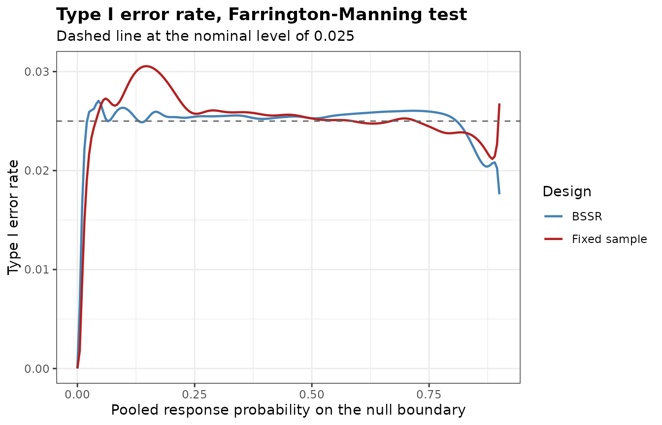
The largest type I error rate is 0.0270 for the re-estimation design,
at
0.045, and 0.0306 for the fixed-sample design, at
0.147. Both exceed the nominal level of 0.025, and the fixed-sample
design exceeds it by more, so the excess comes from the asymptotic test
rather than from the re-estimation. BinaryAlphaAdjBSSR()
accepts margin.scale in the same way and lowers the nominal
level until the rate is controlled.
Tests of equivalence
With alternative = 'equivalence' the null hypothesis
or
is tested against
by two one-sided tests, the test against 'greater' with the
margin
and the test against 'less' with the margin
,
each at the level
.
The margins are given as margin = c(lower, upper), or as a
single value for both. The null hypothesis is rejected when both tests
reject, so the rejection region is the intersection of the two one-sided
regions.
eq <- BinaryRR(N1 = 80, N2 = 80, alpha = 0.05, Test = 'Farrington-Manning',
               alternative = 'equivalence', margin = 0.2)
lo <- BinaryRR(N1 = 80, N2 = 80, alpha = 0.05, Test = 'Farrington-Manning',
               alternative = 'greater', margin = 0.2)
up <- BinaryRR(N1 = 80, N2 = 80, alpha = 0.05, Test = 'Farrington-Manning',
               alternative = 'less', margin = 0.2)
identical(as.vector(eq), as.vector(lo) & as.vector(up))
#> [1] TRUE
The normal approximation to the sample size adds the approximate
powers of the two one-sided tests and subtracts 1, which gives a lower
bound for the approximate probability that both reject, and solves for
the size at which this bound reaches the target power. The exact search
of BinarySampleSize() starts from that size.
plan.eq <- BinarySampleSize(p1 = 0.4, p2 = 0.4, r = 1, alpha = 0.05, tar.power = 0.8,
                            Test = 'Farrington-Manning', alternative = 'equivalence',
                            margin = 0.2)
plan.eq
#> Sample size for a two-arm trial with a binary endpoint
#>
#>   Test             : Farrington-Manning
#>   Alternative      : equivalence
#>   Response rates   : p1 = 0.4, p2 = 0.4
#>   Allocation ratio : 1 to 1
#>   Margin           : -0.2 to 0.2 (risk difference)
#>   Alpha            : 0.05
#>   Target power     : 0.8
#>   Exact search     : crossing
#>
#>   Required sample size: N1 = 101, N2 = 101, total N = 202
#>   Attained power      : 0.8005
In a re-estimation design the assumed difference Delta.A
must lie between the margins, and is usually 0. The type I error rate is
evaluated on both boundaries of the null hypothesis,
and
,
and its largest value is certified on each. For normally distributed
outcomes, Glimm, Yau and Woehling (2021) found that blinded
re-estimation can inflate the type I error rate of a test of equivalence
more than that of a test of superiority, because on a boundary away from
no difference the blinded estimate of the variance depends on the true
difference. For binary outcomes the rate can be computed exactly.
tie.eq <- BinaryTypeIErrorBSSR(
  Delta.A = 0, N1 = plan.eq$N1, N2 = plan.eq$N2, omega = 0.3, r = 1, alpha = 0.05,
  tar.power = 0.8, Test = 'Farrington-Manning', alternative = 'equivalence',
  ss.method = 'standard', margin = 0.2
)
attr(tie.eq, 'max')
#>   Design     theta        TIE      bound boundary
#> 1   BSSR 0.5000000 0.05400202 0.05400202    lower
#> 2   TRAD 0.6342773 0.05352131 0.05352131    lower
plot(tie.eq)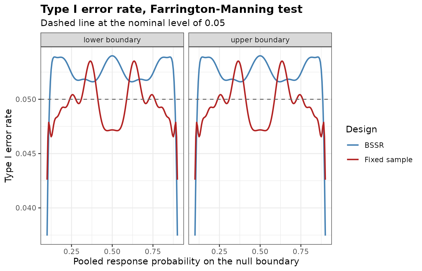
The largest type I error rate is 0.0540 for the re-estimation design
and 0.0535 for the fixed-sample design of 202 patients. The
re-estimation design exceeds the fixed-sample design, and both rates are
computed for the same test of Farrington and Manning, whose fixed-sample
rate already exceeds the level of 0.05. With equal margins and equal
allocation the two boundaries are mirror images and give the same rates.
BinaryAlphaAdjBSSR() lowers the level of both one-sided
tests until the rate is controlled on both boundaries.
adj.eq <- BinaryAlphaAdjBSSR(
  Delta.A = 0, N1 = plan.eq$N1, N2 = plan.eq$N2, omega = 0.3, r = 1, alpha = 0.05,
  tar.power = 0.8, Test = 'Farrington-Manning', alternative = 'equivalence',
  ss.method = 'standard', margin = 0.2
)
adj.eq
#> Adjusted significance level for blinded sample size re-estimation
#>
#>   Test            : Farrington-Manning
#>   Alternative     : equivalence
#>   Adjusted part   : final analysis only
#>   Margin          : -0.2 to 0.2 (risk difference)
#>   Maximum         : certified over theta in [0.1, 0.9] on the lower boundary and [0.1, 0.9] on the upper boundary
#>   Target level    : 0.05
#>
#>        Design   max.TIE alpha.adj max.TIE.adj Boundary
#>          BSSR 0.0540020 0.0467474   0.0496199    lower
#>  Fixed sample 0.0535213 0.0474232   0.0492922    lower
The adjusted level of each one-sided test is 0.0467474 for the re-estimation design and 0.0474232 for the fixed-sample design.
References
Blackwelder, W. C. (1982). “Proving the null hypothesis” in clinical trials. Controlled Clinical Trials, 3, 345-353.
Farrington, C. P. and Manning, G. (1990). Test statistics and sample size formulae for comparative binomial trials with null hypothesis of non-zero risk difference or non-unity relative risk. Statistics in Medicine, 9, 1447-1454.
Friede, T., Mitchell, C. and Mueller-Velten, G. (2007). Blinded sample size reestimation in non-inferiority trials with binary endpoints. Biometrical Journal, 49, 903-916.
Glimm, E., Yau, L. and Woehling, H. (2021). Type I error inflation of blinded sample size re-estimation in equivalence testing. Statistics in Biopharmaceutical Research, 13, 156-169.