Introduction to bbssr

library(bbssr)

What the package does

A trial with a binary endpoint needs an assumed response probability in each group before the first patient is enrolled. If the pooled response probability turns out to differ from what was assumed, the trial ends up either underpowered or larger than it needed to be. Blinded sample size re-estimation addresses this by looking at the pooled number of responders partway through the trial and adjusting the remaining enrolment, without ever splitting the data by treatment group.

The package covers the whole chain of calculations that this requires. Everything rests on BinaryRR(), which returns the rejection region of a test over the grid of possible outcomes. BinaryPower() sums the binomial probability mass over that region, BinarySampleSize() searches, from the normal approximation, for the sample size at which the exact power first attains a target, BinaryPowerBSSR() averages the power over the distribution of the interim data, and BinaryBSSR() applies the re-estimation to a single observed interim data set. BinaryTypeIErrorBSSR() evaluates the type I error rate of a re-estimation design over the nuisance parameter, BinaryAlphaAdjBSSR() lowers the nominal level until that rate is controlled, and BinaryCondRejectBSSR() decomposes the rate by the interim outcome. BinaryGridBSSR() evaluates several designs over common scenarios and returns one data frame.

The seven tests

tests <- c('Chisq', 'Fisher', 'Fisher-midP', 'Z-pool', 'Boschloo')

Chisq is the Pearson chi-squared test without a continuity correction. Fisher is the Fisher exact test and Fisher-midP its mid-p variant. Z-pool and Boschloo are exact unconditional tests, which remove the nuisance parameter by maximizing the null tail probability over the common response probability rather than by conditioning on the total number of responders. Blackwelder and Farrington-Manning are the tests of non-inferiority of Blackwelder (1982) and of Farrington and Manning (1990), which take a margin on the scale of the risk difference, or with margin.scale = 'RR' on the scale of the risk ratio, through the argument margin. With margin = 0 they are tests of superiority, and the Farrington-Manning test then coincides with Chisq. The bbssr-non-inferiority vignette covers these two tests, and the comparisons below use the other five.

Only Fisher, Z-pool and Boschloo keep the type I error rate of a fixed-sample design at or below the nominal level for every value of the nuisance parameter. For the two unconditional tests this holds up to the search over a grid of the nuisance parameter, which ref.pvalue = TRUE refines. The two unconditional tests are slower to compute than Fisher’s test and usually more powerful. The chi-squared and mid-p tests do not carry the guarantee.

Rejection regions

RR <- BinaryRR(N1 = 10, N2 = 10, alpha = 0.025, Test = 'Boschloo')
RR
#> Rejection region for a two-arm trial with a binary endpoint
#> 
#>   Test          : Boschloo
#>   Alternative   : greater
#>   Sample sizes  : N1 = 10, N2 = 10
#>   Alpha         : 0.025
#>   Grid points   : 100
#>   Berger-Boos   : not used
#>   Refinement    : not used
#> 
#>   Rejected outcomes: 23 of 121
#> 
#>       x2=0 x2=1 x2=2 x2=3 x2=4 x2=5 x2=6 x2=7 x2=8 x2=9 x2=10
#> x1=0  .    .    .    .    .    .    .    .    .    .    .    
#> x1=1  .    .    .    .    .    .    .    .    .    .    .    
#> x1=2  .    .    .    .    .    .    .    .    .    .    .    
#> x1=3  .    .    .    .    .    .    .    .    .    .    .    
#> x1=4  X    .    .    .    .    .    .    .    .    .    .    
#> x1=5  X    .    .    .    .    .    .    .    .    .    .    
#> x1=6  X    X    .    .    .    .    .    .    .    .    .    
#> x1=7  X    X    X    .    .    .    .    .    .    .    .    
#> x1=8  X    X    X    X    .    .    .    .    .    .    .    
#> x1=9  X    X    X    X    X    .    .    .    .    .    .    
#> x1=10 X    X    X    X    X    X    X    .    .    .    .    
#> 
#>   X marks rejection of the null hypothesis

plot(RR)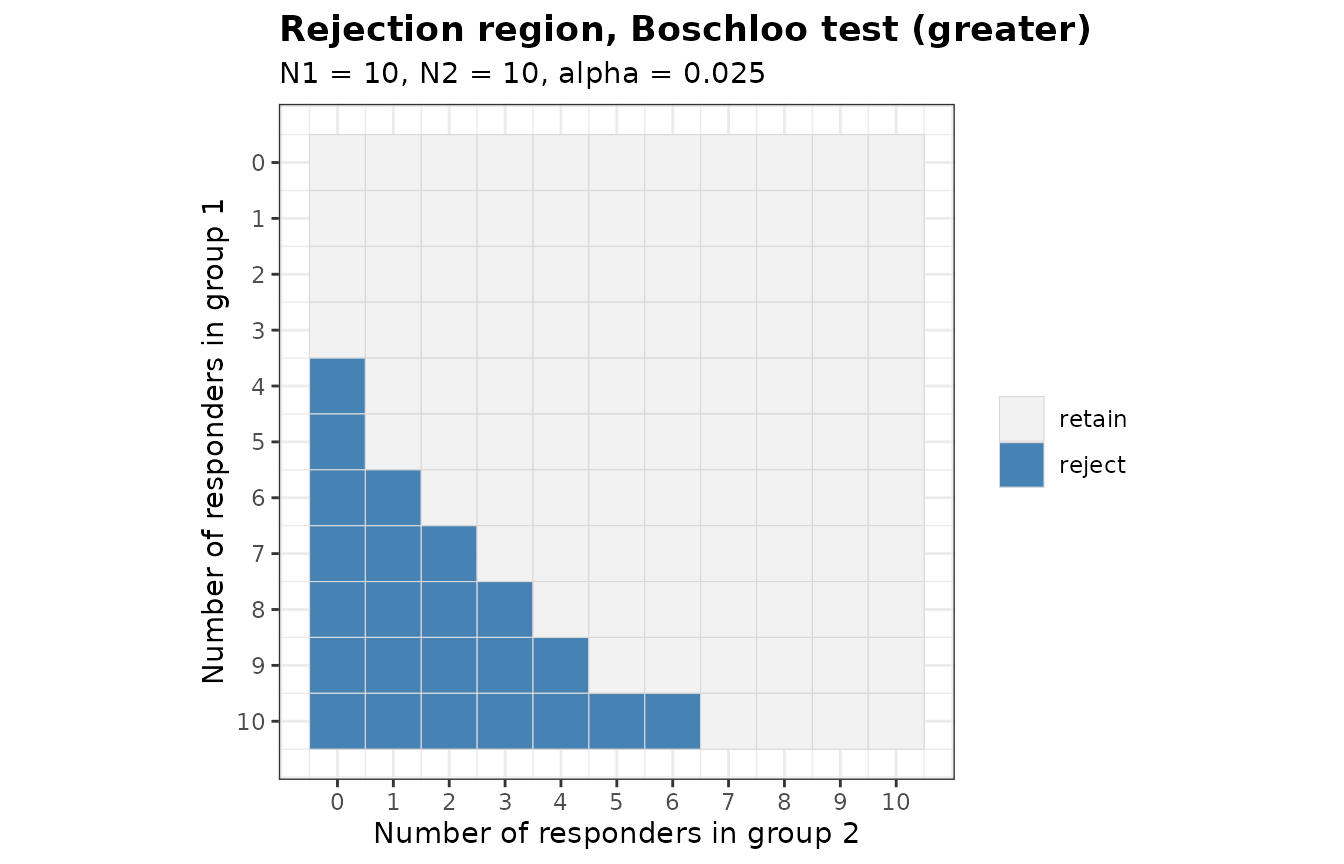

The region is monotone: more responders in group 1, or fewer in group 2, can only move an outcome into the rejection region. Without the Berger-Boos procedure the Boschloo p-value never exceeds the Fisher p-value, so the Boschloo region always contains the Fisher region.

n_rejected <- vapply(tests, function(tst) {
  sum(BinaryRR(10, 10, 0.025, tst))
}, numeric(1))
n_rejected
#>       Chisq      Fisher Fisher-midP      Z-pool    Boschloo 
#>          23          17          23          23          23

Power and sample size

BinaryPower(p1 = 0.6, p2 = 0.3, N1 = 40, N2 = 40, alpha = 0.025, Test = 'Fisher')
#> Exact power for a two-arm trial with a binary endpoint
#> 
#>   Test         : Fisher
#>   Alternative  : greater
#>   Sample sizes : N1 = 40, N2 = 40
#>   Alpha        : 0.025
#> 
#>   p1  p2  Power
#>  0.6 0.3 0.7248

pw <- BinaryPower(p1 = seq(0.35, 0.75, by = 0.05), p2 = rep(0.3, 9),
                  N1 = 40, N2 = 40, alpha = 0.025, Test = 'Fisher')
plot(pw)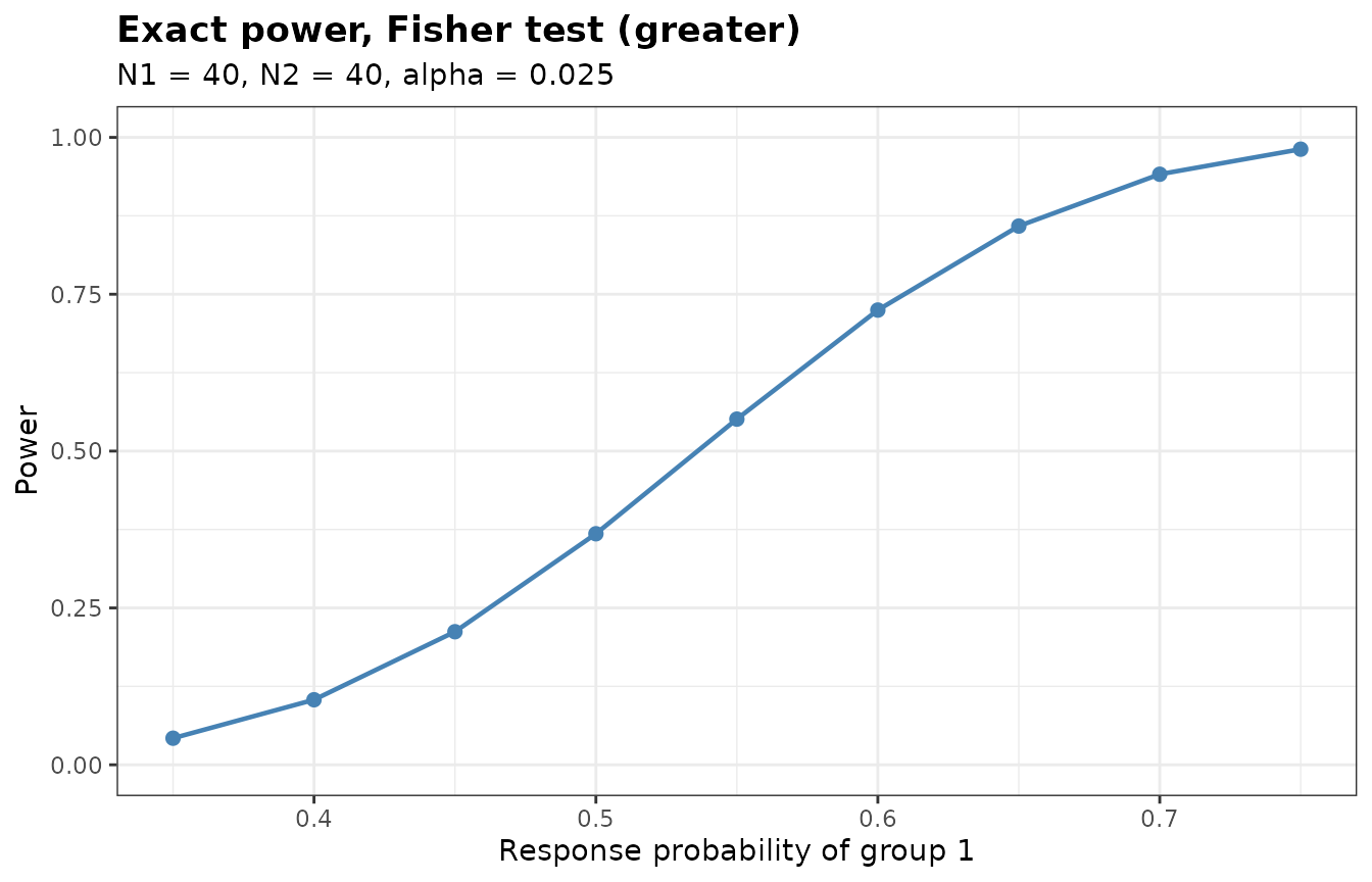

ss <- BinarySampleSize(p1 = 0.6, p2 = 0.3, r = 1, alpha = 0.025,
                       tar.power = 0.8, Test = 'Fisher')
ss
#> Sample size for a two-arm trial with a binary endpoint
#> 
#>   Test             : Fisher
#>   Alternative      : greater
#>   Response rates   : p1 = 0.6, p2 = 0.3
#>   Allocation ratio : 1 to 1
#>   Alpha            : 0.025
#>   Target power     : 0.8
#>   Exact search     : crossing
#> 
#>   Required sample size: N1 = 48, N2 = 48, total N = 96
#>   Attained power      : 0.8005

The exact power is not monotone in the sample size. Adding one patient changes the set of attainable significance levels, and the largest level below alpha can fall rather than rise. The following table shows the effect around the selected sample size.

n2 <- (ss$N2 - 6):(ss$N2 + 5)
data.frame(
  N2 = n2,
  Power = round(vapply(n2, function(n) {
    BinaryPower(0.6, 0.3, n, n, 0.025, 'Fisher')$Power
  }, numeric(1)), 4)
)
#>    N2  Power
#> 1  42 0.7638
#> 2  43 0.7373
#> 3  44 0.7417
#> 4  45 0.7575
#> 5  46 0.7697
#> 6  47 0.7858
#> 7  48 0.8005
#> 8  49 0.8152
#> 9  50 0.8290
#> 10 51 0.8419
#> 11 52 0.8540
#> 12 53 0.8361

This is why the sample size search evaluates the exact power at every candidate it visits rather than inverting a smooth approximation.

The argument search chooses among three searches. The default 'crossing' steps from the normal approximation to a size that attains the target power while the size one patient smaller does not. 'smallest' returns the smallest size that attains the target power, and 'stable' the smallest size from which every size up to a limit attains it, the limit being by default the larger of twice the normal approximation and the normal approximation plus 50. With a target power of 0.85 the three searches give the following sizes of group 2.

searches <- c('crossing', 'smallest', 'stable')
sizes <- vapply(searches, function(s) {
  BinarySampleSize(p1 = 0.6, p2 = 0.3, r = 1, alpha = 0.025, tar.power = 0.85,
                   Test = 'Fisher', search = s)$N2
}, numeric(1))
sizes
#> crossing smallest   stable 
#>       52       52       56

The search 'stable' returns 56 rather than 52 because the power falls below the target again at a size in between.

Blinded sample size re-estimation

p.plan <- c(0.56, 0.26)
p.grid <- seq(0.29, 0.49, by = 0.04)

Consider a trial designed for a response probability of 0.56 in group 1 and 0.26 in group 2, so an assumed treatment effect of 0.3 and a pooled probability of 0.41.

The variance of a binary endpoint is largest at one half, so at a fixed risk difference the required sample size grows as the pooled probability approaches that value. A trial sized at a pooled probability of 0.41 is therefore over-powered if the true value turns out lower, and under-powered if it turns out higher.

plan <- BinarySampleSize(p1 = p.plan[1], p2 = p.plan[2], r = 1, alpha = 0.025,
                         tar.power = 0.8, Test = 'Z-pool')
plan
#> Sample size for a two-arm trial with a binary endpoint
#> 
#>   Test             : Z-pool
#>   Alternative      : greater
#>   Response rates   : p1 = 0.56, p2 = 0.26
#>   Allocation ratio : 1 to 1
#>   Alpha            : 0.025
#>   Target power     : 0.8
#>   Exact search     : crossing
#> 
#>   Required sample size: N1 = 43, N2 = 43, total N = 86
#>   Attained power      : 0.8106

BinaryPowerBSSR() traces both effects. The scenarios below run from a pooled probability of 0.29 up to 0.49, with the design fixed at the sample size above.

res <- BinaryPowerBSSR(
  p = p.grid,
  Delta.A = 0.3, Delta.T = 0.3,
  N1 = plan$N1, N2 = plan$N2, omega = 0.5, r = 1,
  alpha = 0.025, tar.power = 0.8, Test = 'Z-pool'
)
res
#> Blinded sample size re-estimation for a binary endpoint
#> 
#>   Test            : Z-pool
#>   Alternative     : greater
#>   Design rule     : unrestricted
#>   Initial size    : N1 = 43, N2 = 43
#>   Interim fraction: 0.5, giving n1 = 22 and n2 = 22
#>   Treatment effect: assumed 0.3, true 0.3 (risk difference)
#>   Re-estimation   : exact power of Z-pool at level 0.025
#>   Alpha           : 0.025, target power 0.8
#> 
#>     p   p1   p2 power.BSSR power.TRAD  E.N
#>  0.29 0.44 0.14     0.7725     0.8792 69.6
#>  0.33 0.48 0.18     0.7861     0.8562 75.5
#>  0.37 0.52 0.22     0.7951     0.8350 80.2
#>  0.41 0.56 0.26     0.7979     0.8106 83.8
#>  0.45 0.60 0.30     0.7975     0.7913 86.2
#>  0.49 0.64 0.34     0.7971     0.7834 87.3

plot(res)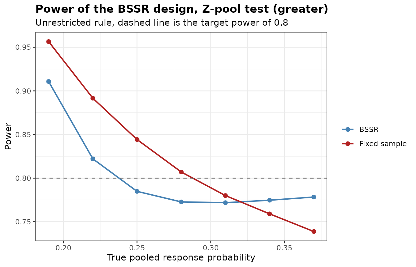

The power.TRAD column falls steadily as the pooled probability rises, from above the target at the low end to below it at the high end. The power.BSSR column stays nearer the target at both ends, since the re-estimation removes patients in the first case and adds them in the second. It lies a little below the target throughout. The E.N column shows the expected total sample size that the re-estimation settles on, against the 86 patients of the fixed design. summary(res) adds the standard deviation and the quartiles of the final total sample size.

Restricted and unrestricted rules

Under the unrestricted rule the trial may end up smaller than planned when the interim data suggest that fewer patients suffice. Under the restricted rule the planned sample size acts as a floor, so the trial can only grow.

args <- list(
  p = seq(0.29, 0.47, by = 0.06),
  Delta.A = 0.3, Delta.T = 0.3, N1 = plan$N1, N2 = plan$N2, omega = 0.5, r = 1,
  alpha = 0.025, tar.power = 0.8, Test = 'Chisq'
)
unrestricted <- do.call(BinaryPowerBSSR, c(args, list(restricted = FALSE)))
restricted <- do.call(BinaryPowerBSSR, c(args, list(restricted = TRUE)))
data.frame(
  p = unrestricted$p,
  power.unrestricted = round(unrestricted$power.BSSR, 4),
  power.restricted = round(restricted$power.BSSR, 4),
  EN.unrestricted = round(unrestricted$E.N, 1),
  EN.restricted = round(restricted$E.N, 1)
)
#>      p power.unrestricted power.restricted EN.unrestricted EN.restricted
#> 1 0.29             0.7828           0.8893            66.4          86.0
#> 2 0.35             0.7870           0.8548            74.3          86.1
#> 3 0.41             0.7934           0.8307            79.8          86.3
#> 4 0.47             0.7982           0.8046            82.9          86.7

For any single interim outcome that calls for more patients than planned the two rules give the same answer, since neither caps the increase. They part company when the interim outcome calls for fewer. The columns above are expectations over all interim outcomes, so they converge rather than coincide as the pooled probability rises. The unrestricted rule takes the saving and ends with a smaller expected trial. The restricted rule keeps at least the planned sample size, which costs patients but never leaves the trial smaller than what the protocol promised.

Re-estimating from observed interim data

The functions above describe a design before the trial starts. Once the trial is running, the interim analysis produces one number that can be shared without unblinding, namely the total count of responders. BinaryBSSR() turns that number into an enrolment decision.

interim <- BinaryBSSR(n1 = ceiling(plan$N1 / 2), n2 = ceiling(plan$N2 / 2), S = 20,
                      Delta.A = 0.3, r = 1, alpha = 0.025, tar.power = 0.8,
                      Test = 'Z-pool')
interim
#> Blinded sample size re-estimation from interim data
#> 
#>   Test             : Z-pool
#>   Alternative      : greater
#>   Design rule      : unrestricted
#>   Assumed effect   : 0.3
#>   Alpha            : 0.025, target power 0.8
#> 
#> Interim data
#>   Patients         : n1 = 22, n2 = 22, total n = 44
#>   Responders       : S = 20, blinded pooled rate = 0.4545
#>   Recovered rates  : hat.p1 = 0.6045, hat.p2 = 0.3045
#> 
#> Re-estimation
#>   Required total   : N1 = 44, N2 = 44, total N = 88
#>   Still to enrol   : group 1 = 22, group 2 = 22, total = 44
#>   Final size       : N1 = 44, N2 = 44, total N = 88
#>   Power at final N : 0.8004

The interim analysis sits at half of the planned 43 patients per group, rounded up. With 20 responders among 44 patients the blinded pooled rate is 0.455, against the assumed 0.41, and the re-estimated total is 88 patients against the 86 of the plan. The bbssr-interim-reestimation vignette works through this in more detail.

Two-sided tests

Every test accepts alternative = 'two.sided'. For the conditional tests, and for the Boschloo test, whose ordering statistic is the Fisher p-value, the two-sided p-value follows one of two conventions, selected with tsmethod.

pw <- function(alpha, alternative, tsmethod = 'minlike') {
  BinaryPower(0.6, 0.3, 40, 40, alpha, 'Fisher',
              alternative = alternative, tsmethod = tsmethod)$Power
}
round(c(
  one.sided.alpha.0.025 = pw(0.025, 'greater'),
  two.sided.alpha.0.025.minlike = pw(0.025, 'two.sided', 'minlike'),
  two.sided.alpha.0.025.central = pw(0.025, 'two.sided', 'central'),
  two.sided.alpha.0.05.minlike = pw(0.05, 'two.sided', 'minlike'),
  two.sided.alpha.0.05.central = pw(0.05, 'two.sided', 'central')
), 4)
#>         one.sided.alpha.0.025 two.sided.alpha.0.025.minlike 
#>                        0.7248                        0.6419 
#> two.sided.alpha.0.025.central  two.sided.alpha.0.05.minlike 
#>                        0.6419                        0.7248 
#>  two.sided.alpha.0.05.central 
#>                        0.7248

At the same nominal level the two-sided test is the less powerful, since half of the level is spent on a direction the alternative does not point in. At twice the level it comes back to the one-sided test, because the lower tail contributes almost nothing to the power when the true effect is positive. With equal group sizes the conditional distribution of the responder count of group 1 is symmetric, so the two conventions give the same power here. With unequal group sizes they can differ, as the bbssr-statistical-methods vignette shows.

The alternative 'less', under which group 1 has the lower response probability, is obtained by exchanging the two groups, so it gives the same power as 'greater' with the groups exchanged.

c(greater = BinaryPower(0.6, 0.3, 40, 40, 0.025, 'Fisher')$Power,
  less = BinaryPower(0.3, 0.6, 40, 40, 0.025, 'Fisher', alternative = 'less')$Power)
#>  greater     less 
#> 0.724766 0.724766

The bbssr-statistical-methods vignette explains the two conventions and the Berger-Boos procedure for the unconditional tests.

Type I error rate of a re-estimation design

BinaryTypeIErrorBSSR() evaluates the rejection probability of the design above under equal response probabilities over a grid of the common value, and finds its largest value over the whole range of the grid together with an upper bound.

tie <- BinaryTypeIErrorBSSR(
  Delta.A = 0.3, N1 = plan$N1, N2 = plan$N2, omega = 0.5, r = 1,
  alpha = 0.025, tar.power = 0.8, Test = 'Z-pool'
)
tie
#> Type I error rate of blinded sample size re-estimation for a binary endpoint
#> 
#>   Test            : Z-pool
#>   Alternative     : greater
#>   Initial size    : N1 = 43, N2 = 43
#>   Interim size    : n1 = 22, n2 = 22
#>   Assumed effect  : 0.3 (RD)
#>   Nominal level   : 0.025
#>   Grid            : 201 values of theta in [0, 1]
#>   Maximum         : certified over theta in [0, 1]
#> 
#> Largest type I error rate
#>        Design    theta     TIE
#>          BSSR 0.103637 0.02344
#>  Fixed sample 0.350533 0.02480

The bbssr-type1-error vignette explains this output and shows how BinaryAlphaAdjBSSR() lowers the nominal level when the rate exceeds it.

Where to go next

bbssr-interim-reestimation follows a single trial from planning to the interim decision.
bbssr-reestimation-rules covers the options of the re-estimation: the normal approximation, the rounding rules, bounds on the final sample size and the risk ratio and odds ratio.
bbssr-design-grid compares several designs with BinaryGridBSSR().
bbssr-non-inferiority covers the tests with a margin and the re-estimation in non-inferiority trials.
bbssr-paired covers matched pairs, such as cross-over trials.
bbssr-stratified covers stratified designs with two or more strata.
bbssr-type1-error covers the type I error rate, the adjusted level and the conditional rejection probabilities.
bbssr-statistical-methods derives the tests and the re-estimation.
bbssr-validation compares the package with stats, Exact, exact2x2 and published results, and reports timings.
bbssr-published-figures redraws published figures from values computed with the package.

References

Blackwelder, W. C. (1982). “Proving the null hypothesis” in clinical trials. Controlled Clinical Trials, 3, 345-353.

Farrington, C. P. and Manning, G. (1990). Test statistics and sample size formulae for comparative binomial trials with null hypothesis of non-zero risk difference or non-unity relative risk. Statistics in Medicine, 9, 1447-1454.

Gosuke Homma

2026-10-28