Options of the Sample Size Re-estimation

library(bbssr)

A reference design

At the interim analysis the blinded pooled response probability is split into two group-specific probabilities with the assumed effect, and the sample size is re-estimated from them. This vignette goes through the arguments that control how this is done. They are shared by BinaryPowerBSSR(), BinaryBSSR(), BinaryTypeIErrorBSSR(), BinaryAlphaAdjBSSR(), BinaryCondRejectBSSR() and BinaryGridBSSR().

The examples use a trial with an assumed risk difference of 0.3, one-to-one allocation, a one-sided level of 0.025, a target power of 0.8 and the chi-squared test in the final analysis. The initial sample size is planned for response probabilities of 0.5 and 0.2, and the interim analysis takes place after half of it.

plan <- BinarySampleSize(p1 = 0.5, p2 = 0.2, r = 1, alpha = 0.025, tar.power = 0.8,
                         Test = 'Chisq')
design <- list(Delta.A = 0.3, N1 = plan$N1, N2 = plan$N2, omega = 0.5, r = 1,
               alpha = 0.025, tar.power = 0.8, Test = 'Chisq')
p.true <- seq(0.2, 0.5, by = 0.1)
plan
#> Sample size for a two-arm trial with a binary endpoint
#> 
#>   Test             : Chisq
#>   Alternative      : greater
#>   Response rates   : p1 = 0.5, p2 = 0.2
#>   Allocation ratio : 1 to 1
#>   Alpha            : 0.025
#>   Target power     : 0.8
#>   Exact search     : crossing
#> 
#>   Required sample size: N1 = 39, N2 = 39, total N = 78
#>   Attained power      : 0.8128

Exact power or the normal approximation

ss.method selects how the sample size is re-estimated from the recovered probabilities.

'exact' (the default) steps from the normal approximation, one patient at a time, to the sample size at which the exact power of the test first attains the target, as BinarySampleSize() does. The argument search replaces this search by the smallest size that attains the target power or by the smallest size from which every size up to a limit attains it, see the bbssr-introduction vignette.
'standard' uses the normal approximation with the variance under the null hypothesis in the term of the significance level and the variance under the alternative in the term of the power, formula (21.3) of Kieser (2020).
'null.variance' uses the variance under the null hypothesis in both terms, formula (1) of Friede and Kieser (2004).
'alternative.variance' uses the variance under the alternative in both terms. With a non-inferiority margin this is the formula of Blackwelder (1982), see the bbssr-non-inferiority vignette.

The bbssr-statistical-methods vignette gives the formulas. The table below shows the final total sample size that each method gives for every fourth value of the pooled number of interim responders s.

methods <- c('exact', 'standard', 'null.variance')
fits <- lapply(methods, function(m) {
  do.call(BinaryPowerBSSR, c(design, list(p = p.true, Delta.T = 0.3, ss.method = m)))
})
names(fits) <- methods
final.total <- function(fit) {
  map <- attr(fit, 'reestimation')
  map$N1 + map$N2
}
map <- attr(fits$exact, 'reestimation')
by.method <- data.frame(s = map$s, hat.p = round(map$hat.p, 3),
                        hat.p1 = round(map$hat.p1, 3), hat.p2 = round(map$hat.p2, 3),
                        exact = final.total(fits$exact),
                        standard = final.total(fits$standard),
                        null.variance = final.total(fits$null.variance))
by.method[seq(1, nrow(by.method), by = 4), ]
#>     s hat.p hat.p1 hat.p2 exact standard null.variance
#> 1   0   0.0   0.15   0.00    72       40            40
#> 5   4   0.1   0.25   0.00    42       40            40
#> 9   8   0.2   0.35   0.05    48       54            56
#> 13 12   0.3   0.45   0.15    68       72            74
#> 17 16   0.4   0.55   0.25    80       82            84
#> 21 20   0.5   0.65   0.35    88       86            88
#> 25 24   0.6   0.75   0.45    80       82            84
#> 29 28   0.7   0.85   0.55    68       72            74
#> 33 32   0.8   0.95   0.65    48       54            56
#> 37 36   0.9   1.00   0.75    42       40            40
#> 41 40   1.0   1.00   0.85    72       40            40

The exact search uses the exact power of the chosen test, so it depends on the test of the final analysis, whereas the two formulas do not. At the lowest interim outcomes the recovered probability of group 2 would be negative, and at the highest that of group 1 would exceed one. The exact search needs probabilities inside the unit interval and truncates them to it, which is what the columns hat.p1 and hat.p2 show. The truncation shrinks the recovered difference, which is why the exact column rises again at both ends. The formulas use the recovered probabilities before truncation, with each Bernoulli variance truncated at zero, so that the assumed difference is kept as in formula (2) of Friede and Kieser (2004).

The power and the expected total sample size of the three versions are as follows.

data.frame(
  p = p.true,
  power.exact = round(fits$exact$power.BSSR, 4),
  power.standard = round(fits$standard$power.BSSR, 4),
  power.null.variance = round(fits$null.variance$power.BSSR, 4),
  E.N.exact = round(fits$exact$E.N, 1),
  E.N.standard = round(fits$standard$E.N, 1),
  E.N.null.variance = round(fits$null.variance$E.N, 1)
)
#>     p power.exact power.standard power.null.variance E.N.exact E.N.standard
#> 1 0.2      0.7875         0.8138              0.8244      50.6         54.3
#> 2 0.3      0.7784         0.7984              0.8058      67.5         70.3
#> 3 0.4      0.7936         0.8031              0.8089      78.5         80.4
#> 4 0.5      0.8023         0.8037              0.8006      81.9         83.7
#>   E.N.null.variance
#> 1              56.3
#> 2              72.4
#> 3              82.6
#> 4              86.2

Another test or level for the re-estimation

By default the sample size is re-estimated with the test and the level of the final analysis. ss.Test gives another test for the exact search, and ss.alpha another level. A final analysis with the Boschloo test can, for example, re-estimate the sample size with the exact power of the chi-squared test, which is quicker to search over. The chi-squared test does not keep the nominal level and attains the target power with fewer patients than the Boschloo test, so the sizes it gives are smaller, and the power of the Boschloo test falls further below the target, as the table shows.

boschloo <- modifyList(design, list(Test = 'Boschloo'))
fit.boschloo <- do.call(BinaryPowerBSSR, c(boschloo, list(p = p.true, Delta.T = 0.3)))
fit.chisq <- do.call(BinaryPowerBSSR,
                     c(boschloo, list(p = p.true, Delta.T = 0.3, ss.Test = 'Chisq')))
data.frame(
  p = p.true,
  power.ss.Boschloo = round(fit.boschloo$power.BSSR, 4),
  power.ss.Chisq = round(fit.chisq$power.BSSR, 4),
  E.N.ss.Boschloo = round(fit.boschloo$E.N, 1),
  E.N.ss.Chisq = round(fit.chisq$E.N, 1)
)
#>     p power.ss.Boschloo power.ss.Chisq E.N.ss.Boschloo E.N.ss.Chisq
#> 1 0.2            0.7946         0.7587            55.9         50.6
#> 2 0.3            0.7809         0.7577            71.2         67.5
#> 3 0.4            0.7943         0.7780            82.2         78.5
#> 4 0.5            0.7925         0.7617            86.5         81.9

ss.alpha matters when the final analysis uses an adjusted level. BinaryAlphaAdjBSSR() with adjust = 'test' lowers the level of the final analysis only, so the re-estimation keeps ss.alpha, and with adjust = 'both' it lowers both, see the bbssr-type1-error vignette.

Whole numbers

The normal approximation gives an unrounded sample size, and rounding turns it into whole numbers.

'group' (the default) rounds up the size of group 2 and gives group 1 ceiling(r * N2) patients. It is the only rule available with ss.method = 'exact'.
'friede-kieser' gives the second stage the rounded-up excess of the unrounded total over the interim total, split into ceiling(n / (1 + r)) and ceiling(r * n / (1 + r)) patients as in Friede and Kieser (2004).
'total' rounds up the total and gives group 2 floor(N / (1 + r)) patients.
'nearest' rounds each group to the nearest whole number, as in Farrington and Manning (1990).

With an allocation ratio of 2 to 1 the four rules give the following final sample sizes for one interim outcome.

rounding.rules <- c('group', 'friede-kieser', 'total', 'nearest')
do.call(rbind, lapply(rounding.rules, function(rule) {
  b <- BinaryBSSR(n1 = 30, n2 = 15, S = 18, Delta.A = 0.25, r = 2, alpha = 0.025,
                  tar.power = 0.8, Test = 'Chisq', ss.method = 'standard',
                  rounding = rule)
  data.frame(rounding = rule, N1.final = b$N1.final, N2.final = b$N2.final,
             N.final = b$N.final)
}))
#>        rounding N1.final N2.final N.final
#> 1         group       88       44     132
#> 2 friede-kieser       87       44     131
#> 3         total       87       43     130
#> 4       nearest       86       43     129

Bounds on the final sample size

The final total sample size is never smaller than the interim total. Three arguments add further bounds. restricted = TRUE keeps the initial sample size as a lower bound, so the trial can only grow. N.min is a lower bound on the total, which can keep the patients who are already enrolled but not yet evaluated at the interim analysis. N.max is an upper bound on the total. Below it is set to the initial total, so that the trial can only shrink, which is the mirror image of the restricted rule. Under the rounding rules 'friede-kieser' and 'nearest', which round the two groups separately, the total can exceed N.max by one patient.

bounds <- list(unrestricted = list(), restricted = list(restricted = TRUE),
               capped = list(N.max = plan$N))
do.call(rbind, lapply(names(bounds), function(nm) {
  fit <- do.call(BinaryPowerBSSR, c(design, list(p = p.true, Delta.T = 0.3,
                                                 ss.method = 'standard'),
                                    bounds[[nm]]))
  s <- summary(fit)
  data.frame(rule = nm, p = s$p, power.BSSR = round(fit$power.BSSR, 4),
             E.N = round(s$E.N, 1), N.q50 = s$N.q50, P.N.max = round(s$P.N.max, 3))
}))
#>            rule   p power.BSSR  E.N N.q50 P.N.max
#> 1  unrestricted 0.2     0.8138 54.3    54   0.000
#> 2  unrestricted 0.3     0.7984 70.3    72   0.010
#> 3  unrestricted 0.4     0.8031 80.4    82   0.165
#> 4  unrestricted 0.5     0.8037 83.7    84   0.381
#> 5    restricted 0.2     0.9509 78.0    78   0.000
#> 6    restricted 0.3     0.8543 78.7    78   0.010
#> 7    restricted 0.4     0.8111 81.7    82   0.165
#> 8    restricted 0.5     0.8047 83.9    84   0.381
#> 9        capped 0.2     0.8138 54.3    54   0.012
#> 10       capped 0.3     0.7962 69.6    72   0.287
#> 11       capped 0.4     0.7803 76.7    78   0.801
#> 12       capped 0.5     0.7768 77.9    78   0.970

P.N.max is the probability that the final total takes the largest value that any interim outcome leads to. When the cap binds, this is the probability of ending at the cap, or one patient below it when the cap cannot be split in the ratio r to 1.

Interim sample sizes

omega gives the interim analysis as a fraction of the initial sample size. Group 2 then has ceiling(omega * N2) patients at the interim analysis and group 1 has ceiling(r * ceiling(omega * N2)), so the interim analysis keeps the allocation ratio. n.interim gives the two interim sample sizes directly instead, for example when the interim analysis is triggered by a number of evaluated patients.

c(n1.interim = attr(fits$exact, 'n1.interim'),
  n2.interim = attr(fits$exact, 'n2.interim'))
#> n1.interim n2.interim 
#>         20         20
fit.interim <- do.call(BinaryPowerBSSR,
                       c(modifyList(design, list(omega = NULL)),
                         list(p = p.true, Delta.T = 0.3, n.interim = c(20, 15))))
c(n1.interim = attr(fit.interim, 'n1.interim'),
  n2.interim = attr(fit.interim, 'n2.interim'))
#> n1.interim n2.interim 
#>         20         15

Risk ratio and odds ratio

The assumed effect Delta.A and the true effect Delta.T are risk differences by default. With effect = 'RR' they are risk ratios p1 / p2, and the recovered probabilities are those with the pooled value $\hat{p}$ and the ratio Delta.A, formula (21.11) of Kieser (2020). With effect = 'OR' they are odds ratios, and the recovered probabilities are obtained from the quadratic equation that the odds ratio and the pooled value define. The same interim data give the following recovered probabilities and re-estimated sample sizes on the three scales.

effects <- data.frame(effect = c('RD', 'RR', 'OR'), Delta.A = c(0.2, 2.5, 3),
                      stringsAsFactors = FALSE)
do.call(rbind, lapply(seq_len(nrow(effects)), function(i) {
  b <- BinaryBSSR(n1 = 20, n2 = 20, S = 12, Delta.A = effects$Delta.A[i], r = 1,
                  alpha = 0.025, tar.power = 0.8, Test = 'Chisq',
                  effect = effects$effect[i])
  data.frame(effect = effects$effect[i], Delta.A = effects$Delta.A[i],
             hat.p = b$hat.p, hat.p1 = round(b$hat.p1, 4), hat.p2 = round(b$hat.p2, 4),
             N.re = b$N.re)
}))
#>   effect Delta.A hat.p hat.p1 hat.p2 N.re
#> 1     RD     0.2   0.3 0.4000 0.2000  160
#> 2     RR     2.5   0.3 0.4286 0.1714   96
#> 3     OR     3.0   0.3 0.4112 0.1888  130

Distribution of the final sample size

BinaryPowerBSSR() reports the expected final total sample size E.N. summary() adds its standard deviation, its quartiles and the probability that it reaches the largest attainable value, and the attribute N.dist holds the whole distribution for every scenario.

summary(fits$exact)
#>     p1   p2   p      E.N      SD.N N.q25 N.q50 N.q75      P.N.max
#> 1 0.35 0.05 0.2 50.58920 10.156191    42    48    62 2.145897e-06
#> 2 0.45 0.15 0.3 67.48905 10.782479    62    68    78 2.567452e-03
#> 3 0.55 0.25 0.4 78.52342  6.195798    78    80    82 5.358597e-02
#> 4 0.65 0.35 0.5 81.92035  3.289272    82    82    82 1.315918e-01
n.dist <- attr(fits$exact, 'N.dist')
head(n.dist)
#>   scenario   p N1 N2  N       prob
#> 1        1 0.2 20 20 40 0.20553366
#> 2        1 0.2 21 21 42 0.20020920
#> 3        1 0.2 24 24 48 0.18408246
#> 4        1 0.2 27 27 54 0.15362938
#> 5        1 0.2 31 31 62 0.11309921
#> 6        1 0.2 33 33 66 0.07228451

library(ggplot2)

ggplot(n.dist, aes(x = N, y = prob)) +
  geom_col() +
  facet_wrap(~ p, labeller = label_both) +
  labs(x = 'Final total sample size', y = 'Probability') +
  theme_bw()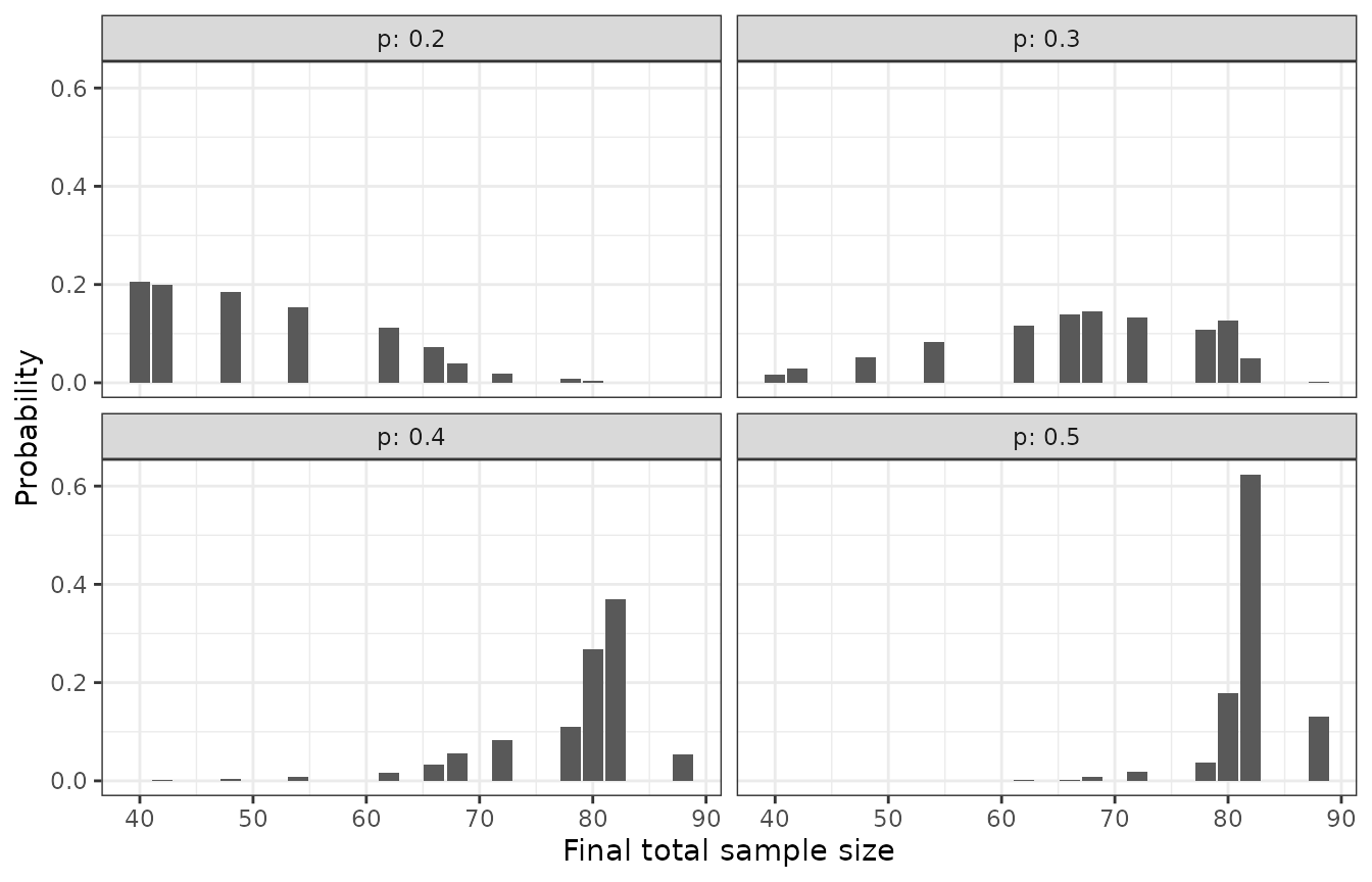

References

Blackwelder, W. C. (1982). “Proving the null hypothesis” in clinical trials. Controlled Clinical Trials, 3, 345-353.

Farrington, C. P. and Manning, G. (1990). Test statistics and sample size formulae for comparative binomial trials with null hypothesis of non-zero risk difference or non-unity relative risk. Statistics in Medicine, 9, 1447-1454.

Friede, T. and Kieser, M. (2004). Sample size recalculation for binary data in internal pilot study designs. Pharmaceutical Statistics, 3, 269-279.

Kieser, M. (2020). Methods and Applications of Sample Size Calculation and Recalculation in Clinical Trials. Springer.

Gosuke Homma

2026-10-28