Plot Exact Power against the Response Probability of Group 1

Usage

# S3 method for class 'bbssr_power'
plot(
  x,
  main = NULL,
  sub = NULL,
  xlab = NULL,
  ylab = NULL,
  ylim = c(0, 1),
  show.points = TRUE,
  colours = NULL,
  base_size = 11,
  ...
)

Arguments

x: An object of class bbssr_power returned by BinaryPower
main: Title of the plot. The default of NULL builds the title from the object and a single NA drops it
sub: Subtitle of the plot, following the convention of main
xlab: Label of the horizontal axis, following the convention of main
ylab: Label of the vertical axis, following the convention of main
ylim: Numeric vector of length two giving the range of the vertical axis, or NULL for a range chosen from the data
show.points: Logical. If TRUE, the default, a marker is drawn at every evaluated response probability. Set it to FALSE to draw the curve alone, which is easier to read on a fine grid
colours: Colour of the curve
base_size: Base font size of the theme, in points
...: Further arguments, currently ignored

Value

A ggplot object

Details

The vertical range is imposed with coord_cartesian, so points outside ylim are hidden rather than removed from the data.

Examples

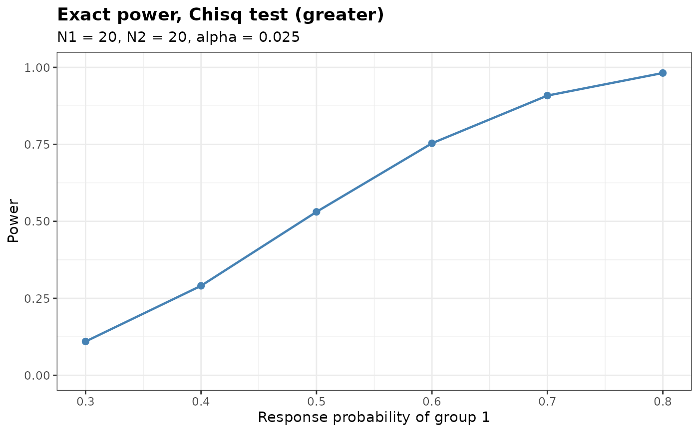
pw <- BinaryPower(p1 = seq(0.3, 0.8, by = 0.1), p2 = rep(0.2, 6),
                  N1 = 20, N2 = 20, alpha = 0.025, Test = 'Chisq')
plot(pw)


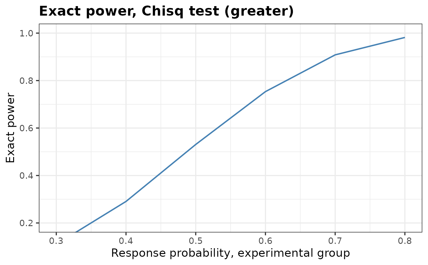
# Enlarge the type, rescale the vertical axis, rename the axes and drop the markers
plot(pw, base_size = 14, ylim = c(0.2, 1), sub = NA, show.points = FALSE,
     xlab = 'Response probability, experimental group', ylab = 'Exact power')