Power of a Blinded Sample Size Re-estimation Design for Binary Endpoints

Calculates the power of a two-arm trial with a binary endpoint when blinded sample size re-estimation (BSSR) is implemented, together with the power of the corresponding fixed-sample design, the expected final sample size and its distribution. Seven tests are supported (see BinaryRR), each of which can be applied with a one-sided or a two-sided alternative, under either a restricted or an unrestricted design rule.

Usage

BinaryPowerBSSR(
  p,
  Delta.A,
  Delta.T,
  N1,
  N2,
  omega = NULL,
  r,
  alpha,
  tar.power,
  Test,
  restricted = FALSE,
  alternative = c("greater", "less", "two.sided", "equivalence"),
  tsmethod = c("minlike", "central", "blaker"),
  n.grid = 100,
  bb.gamma = 0,
  effect = c("RD", "RR", "OR"),
  ss.method = c("exact", "standard", "null.variance", "alternative.variance"),
  ss.Test = Test,
  ss.alpha = alpha,
  rounding = c("group", "friede-kieser", "total", "nearest"),
  search = c("crossing", "smallest", "stable"),
  search.limit = c(2, 50),
  N.min = NULL,
  N.max = NULL,
  n.interim = NULL,
  margin = 0,
  ref.pvalue = FALSE,
  margin.scale = c("RD", "RR")
)

Arguments

p: Vector of true pooled proportions of responders from both groups
Delta.A: Assumed treatment effect, on the scale given by effect, used to split the blinded pooled proportion into group-specific proportions
Delta.T: True treatment effect, on the scale given by effect
N1: Initial sample size of group 1
N2: Initial sample size of group 2
omega: Fraction of the initial sample size observed at the interim analysis. The interim size of group 2 is ceiling(omega N2) and that of group 1 is ceiling(r ceiling(omega N2)), so the interim analysis keeps the allocation ratio. Either omega or n.interim must be supplied
r: Allocation ratio to group 1
alpha: Level of significance of the final analysis, for the alternative specified by alternative
tar.power: Target power
Test: Type of statistical test of the final analysis. Options: 'Chisq', 'Fisher', 'Fisher-midP', 'Z-pool', 'Boschloo', 'Blackwelder' or 'Farrington-Manning'
restricted: Logical. If TRUE, the re-estimated sample size is not allowed to fall below the initial sample size. Default is FALSE
alternative: Direction of the alternative hypothesis. Options: 'greater' (default), 'less', 'two.sided', or 'equivalence' for the alternative that the effect lies between the margins of a test of equivalence, see margin
tsmethod: Convention used to construct the two-sided version of the conditional tests, see BinaryRR. Options: 'minlike' (default), 'central' or 'blaker'
n.grid: Number of grid points used to search over the nuisance parameter of the unconditional tests. Default is 100
bb.gamma: Confidence level parameter of the Berger-Boos procedure. The default of 0 disables the procedure
effect: Scale of Delta.A and Delta.T. Options: 'RD' (default) for the risk difference p1 - p2, 'RR' for the risk ratio p1 / p2 or 'OR' for the odds ratio
ss.method: How the sample size is re-estimated from the recovered proportions. Options: 'exact' (default), 'standard', 'null.variance' or 'alternative.variance', as in BinarySampleSize
ss.Test: Test whose exact power is used for the re-estimation when ss.method = 'exact'. Default is Test
ss.alpha: Level of significance used for the re-estimation. Default is alpha
rounding: How the re-estimated sample size is turned into whole numbers. Options: 'group' (default), 'friede-kieser', 'total' or 'nearest'. Only 'group' is available with ss.method = 'exact'. See Details
search: How the exact re-estimation chooses the sample size when ss.method = 'exact': 'crossing' (default), 'smallest' or 'stable', as in BinarySampleSize, without going beyond the largest size that N.max allows. Ignored by the other methods
search.limit: Limit of the size of group 2 examined by search = 'stable', as in BinarySampleSize. Default is c(2, 50)
N.min: Lower bound on the final total sample size, or NULL (default) for none beyond the interim total. It can be used to keep the patients who are already enrolled but not yet evaluated at the interim analysis
N.max: Upper bound on the final total sample size, or NULL (default) for none
n.interim: Interim sample sizes of group 1 and group 2, as a vector of length two. An alternative to omega
margin: Non-inferiority margin, on the scale given by margin.scale. On the scale of the risk difference the default of 0 gives a test of superiority, and a value other than 0 tests the null hypothesis p1 - p2 <= -margin against p1 - p2 > -margin when alternative is 'greater', and p1 - p2 >= margin against p1 - p2 < margin when it is 'less'. A negative value tests for superiority by more than its absolute value. On the scale of the risk ratio the margin is a positive ratio R0, and the null hypothesis is p1 / p2 <= R0 against p1 / p2 > R0 when alternative is 'greater', and p1 / p2 >= R0 against p1 / p2 < R0 when it is 'less'. A margin other than 0, and any margin on the scale of the risk ratio, requires Test = 'Blackwelder' or 'Farrington-Manning' and a one-sided alternative or 'equivalence', see BinaryRR. With a margin other than 0 on the scale of the risk difference the assumed and the true effects are risk differences (effect = 'RD'), and with a margin on the scale of the risk ratio they are risk ratios (effect = 'RR'). For alternative = 'equivalence' the margin is the pair c(lower, upper) of margins of a test of equivalence, or a single value used for both. On the scale of the risk difference both margins lie in (0, 1), and the null hypothesis p1 - p2 <= -lower or p1 - p2 >= upper is tested against -lower < p1 - p2 < upper. On the scale of the risk ratio the pair satisfies 0 < lower < 1 < upper, a single ratio R gives the pair of R and 1 / R, the smaller as lower, and the null hypothesis is p1 / p2 <= lower or p1 / p2 >= upper. The null hypothesis is rejected when both one-sided tests reject, each at the level alpha
ref.pvalue: Logical. If TRUE, the maximization over the nuisance parameter of the unconditional tests is refined between the grid points, see BinaryRR. Default is FALSE. It applies to the final analysis, to the fixed-sample comparator and to the exact re-estimation
margin.scale: Scale of margin. Options: 'RD' (default) for the risk difference p1 - p2 or 'RR' for the risk ratio p1 / p2

Value

An object of class bbssr_powerbssr, a data frame with one row per element of p containing:

p1: True probability of responders for group 1
p2: True probability of responders for group 2
p: True pooled probability of responders from both groups
power.BSSR: Power of the BSSR design
power.TRAD: Power of the fixed-sample design
E.N: Expected total sample size of the BSSR design

The interim sample sizes are stored as the attributes n1.interim and n2.interim. The attribute reestimation holds, for every pooled number of interim responders s, the recovered proportions, the final sample sizes and, in the column N2.limit, the limit of search = 'stable' (otherwise NA). The attribute N.dist holds the distribution of the final sample size for every row of the result, identified by the column scenario, and the attribute search the search. summary() reports the standard deviation and quantiles of the final sample size.

Details

At the interim analysis the pooled number of responders is observed without unblinding. The pooled proportion is combined with the assumed treatment effect Delta.A to recover group-specific proportions, from which the sample size is re-estimated. For the risk difference the recovered proportions are hat.p + Delta.A / (1 + r) and hat.p - r Delta.A / (1 + r). For the risk ratio they are the proportions with the pooled value hat.p and the ratio Delta.A, formula (21.11) of Kieser (2020), and for the odds ratio they are obtained from the quadratic equation that the odds ratio and the pooled value define. The exact search of ss.method = 'exact' uses the recovered proportions truncated to the unit interval. The normal approximation uses them before truncation, with each Bernoulli variance truncated at zero, so that the assumed effect is kept as in formula (2) of Friede and Kieser (2004). The power is then averaged over the distribution of the interim outcome.

Under rounding = 'group', both the interim and the final sample size of group 1 are obtained from the size of group 2 by a single application of ceiling(r ...), so the allocation ratio is preserved as closely as whole numbers allow and is exact whenever r is a whole number. Under rounding = 'friede-kieser', which requires a normal approximation, that is an ss.method other than 'exact', the second stage receives the rounded-up excess of the unrounded re-estimated total over the interim total, split into ceiling(n / (1 + r)) and ceiling(r n / (1 + r)) patients as in Friede and Kieser (2004). Under rounding = 'total' the unrounded total is rounded up and group 2 receives floor(N / (1 + r)) patients. Under rounding = 'nearest' the unrounded total is split in the ratio r to 1 and each group is rounded to the nearest whole number, which reproduces the computations of Friede et al. (2007). In each case the final total is kept between the interim total (or N.min, or the initial total under the restricted rule) and N.max, except that 'friede-kieser' and 'nearest' round the two groups separately and can exceed N.max by one patient. The argument N1 enters only through the fixed-sample comparator and the restricted rule, and under rounding = 'group' a warning is issued when it is not ceiling(r N2).

Recovered proportions that coincide admit no sample size. The risk ratio produces them when no interim patient responds, and the odds ratio when no interim patient or every interim patient responds. The initial sample size is kept for such interim outcomes.

Setting Delta.T to the null value (0 for the risk difference, 1 for a ratio) makes the two groups identical, so power.BSSR and power.TRAD become rejection probabilities under the null hypothesis. BinaryTypeIErrorBSSR evaluates them over the unit interval and locates the maximum.

With a non-inferiority margin, the design of Friede et al. (2007) is obtained. The assumed effect Delta.A is usually 0, which recovers the pooled proportion for both groups, the sample size is re-estimated by the formula of Farrington and Manning (ss.method = 'standard') or of Blackwelder (ss.method = 'alternative.variance'), and Delta.T = -margin (or margin for alternative = 'less') gives the rejection probability on the boundary of the null hypothesis.

With margin.scale = 'RR' the margin is a ratio R0 and the effects are risk ratios (effect = 'RR'). The assumed effect Delta.A must exceed R0 for alternative = 'greater' and fall below it for 'less', and is usually 1. The sample size is re-estimated by formula (8) of Farrington and Manning (1990) (ss.method = 'standard') or by their Method 1 (ss.method = 'alternative.variance'), and Delta.T = R0 gives the rejection probability on the boundary of the null hypothesis. The recovered proportions lie on that boundary only when no interim patient responds, and the initial sample size is kept for this interim outcome.

References

Friede T, Kieser M (2004). Sample size recalculation for binary data in internal pilot study designs. Pharmaceutical Statistics, 3(4), 269-279.

Kieser M (2020). Methods and Applications of Sample Size Calculation and Recalculation in Clinical Trials. Springer, Cham.

Friede T, Mitchell C, Mueller-Velten G (2007). Blinded sample size reestimation in non-inferiority trials with binary endpoints. Biometrical Journal, 49(6), 903-916.

Author

Gosuke Homma (my.name.is.gosuke@gmail.com)

Examples

# Small BSSR calculation with the chi-squared test
BinaryPowerBSSR(
  p = 0.45,
  Delta.A = 0.3, Delta.T = 0.3,
  N1 = 5, N2 = 5, omega = 0.5, r = 1,
  alpha = 0.025, tar.power = 0.8, Test = 'Chisq'
)
#> Blinded sample size re-estimation for a binary endpoint
#> 
#>   Test            : Chisq
#>   Alternative     : greater
#>   Design rule     : unrestricted
#>   Initial size    : N1 = 5, N2 = 5
#>   Interim fraction: 0.5, giving n1 = 3 and n2 = 3
#>   Treatment effect: assumed 0.3, true 0.3 (risk difference)
#>   Re-estimation   : exact power of Chisq at level 0.025
#>   Alpha           : 0.025, target power 0.8
#> 
#>     p  p1  p2 power.BSSR power.TRAD  E.N
#>  0.45 0.6 0.3      0.719     0.1667 73.3

# \donttest{
res <- BinaryPowerBSSR(
  p = seq(0.23, 0.47, by = 0.04),
  Delta.A = 0.3, Delta.T = 0.3,
  N1 = 39, N2 = 39, omega = 0.5, r = 1,
  alpha = 0.025, tar.power = 0.8, Test = 'Z-pool'
)
print(res)
#> Blinded sample size re-estimation for a binary endpoint
#> 
#>   Test            : Z-pool
#>   Alternative     : greater
#>   Design rule     : unrestricted
#>   Initial size    : N1 = 39, N2 = 39
#>   Interim fraction: 0.5, giving n1 = 20 and n2 = 20
#>   Treatment effect: assumed 0.3, true 0.3 (risk difference)
#>   Re-estimation   : exact power of Z-pool at level 0.025
#>   Alpha           : 0.025, target power 0.8
#> 
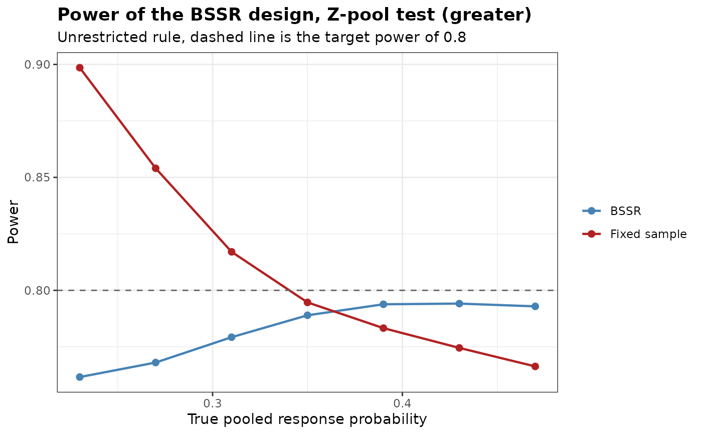
#>     p   p1   p2 power.BSSR power.TRAD  E.N
#>  0.23 0.38 0.08     0.7616     0.8986 58.9
#>  0.27 0.42 0.12     0.7680     0.8540 66.0
#>  0.31 0.46 0.16     0.7793     0.8170 72.2
#>  0.35 0.50 0.20     0.7890     0.7947 77.3
#>  0.39 0.54 0.24     0.7938     0.7833 81.3
#>  0.43 0.58 0.28     0.7941     0.7745 84.3
#>  0.47 0.62 0.32     0.7929     0.7663 86.1
summary(res)
#>     p1   p2    p      E.N      SD.N N.q25 N.q50 N.q75      P.N.max
#> 1 0.38 0.08 0.23 58.88554 11.649441    48    58    68 0.0001982757
#> 2 0.42 0.12 0.27 65.95004 11.429154    58    68    78 0.0024283233
#> 3 0.46 0.16 0.31 72.15765 10.234978    68    72    80 0.0147041223
#> 4 0.50 0.20 0.35 77.26530  8.670204    72    80    82 0.0544992365
#> 5 0.54 0.24 0.39 81.31440  7.112108    80    82    86 0.1380835921
#> 6 0.58 0.28 0.43 84.31936  5.648214    80    86    90 0.2546182696
#> 7 0.62 0.32 0.47 86.11909  4.435730    82    88    90 0.3540672752
plot(res)


# Re-estimation by the normal approximation with an upper bound of twice the
# initial sample size, and a final analysis with the Boschloo test
BinaryPowerBSSR(
  p = seq(0.2, 0.4, by = 0.05),
  Delta.A = 0.3, Delta.T = 0.3,
  N1 = 30, N2 = 30, n.interim = c(15, 15), r = 1,
  alpha = 0.025, tar.power = 0.8, Test = 'Boschloo',
  ss.method = 'standard', N.max = 120
)
#> Blinded sample size re-estimation for a binary endpoint
#> 
#>   Test            : Boschloo
#>   Alternative     : greater
#>   Design rule     : unrestricted
#>   Initial size    : N1 = 30, N2 = 30
#>   Interim size    : n1 = 15 and n2 = 15
#>   Treatment effect: assumed 0.3, true 0.3 (risk difference)
#>   Re-estimation   : normal approximation (standard), group rounding at level 0.025, N.max = 120
#>   Alpha           : 0.025, target power 0.8
#> 
#>     p   p1   p2 power.BSSR power.TRAD  E.N
#>  0.20 0.35 0.05     0.7281     0.8329 53.4
#>  0.25 0.40 0.10     0.7487     0.7431 62.0
#>  0.30 0.45 0.15     0.7606     0.6915 69.5
#>  0.35 0.50 0.20     0.7748     0.6708 75.5
#>  0.40 0.55 0.25     0.7790     0.6596 79.8

# Non-inferiority with a margin of 0.1, as in Friede et al. (2007)
BinaryPowerBSSR(
  p = c(0.5, 0.7), Delta.A = 0, Delta.T = 0,
  N1 = 329, N2 = 329, n.interim = c(66, 66), r = 1,
  alpha = 0.025, tar.power = 0.8, Test = 'Farrington-Manning',
  ss.method = 'standard', rounding = 'nearest', margin = 0.1
)
#> Blinded sample size re-estimation for a binary endpoint
#> 
#>   Test            : Farrington-Manning
#>   Alternative     : greater
#>   Design rule     : unrestricted
#>   Initial size    : N1 = 329, N2 = 329
#>   Interim size    : n1 = 66 and n2 = 66
#>   Treatment effect: assumed 0, true 0 (risk difference)
#>   Margin          : 0.1
#>   Re-estimation   : normal approximation (standard), nearest rounding at level 0.025
#>   Alpha           : 0.025, target power 0.8
#> 
#>    p  p1  p2 power.BSSR power.TRAD   E.N
#>  0.5 0.5 0.5     0.7949     0.7209 773.8
#>  0.7 0.7 0.7     0.7971     0.8006 652.9
# }