Type I Error Rate of a Blinded Sample Size Re-estimation Design

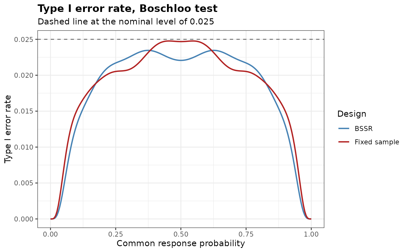
Evaluates the type I error rate of a two-arm trial with a binary endpoint and blinded sample size re-estimation (BSSR) over the common response probability, or over the pooled response probability on the boundary of a non-inferiority hypothesis, together with that of the corresponding fixed-sample design, and locates the largest value of each.

Usage

BinaryTypeIErrorBSSR(
  Delta.A,
  N1,
  N2,
  omega = NULL,
  r,
  alpha,
  tar.power,
  Test,
  restricted = FALSE,
  alternative = c("greater", "less", "two.sided", "equivalence"),
  tsmethod = c("minlike", "central", "blaker"),
  n.grid = 100,
  bb.gamma = 0,
  effect = c("RD", "RR", "OR"),
  ss.method = c("exact", "standard", "null.variance", "alternative.variance"),
  ss.Test = Test,
  ss.alpha = alpha,
  rounding = c("group", "friede-kieser", "total", "nearest"),
  search = c("crossing", "smallest", "stable"),
  search.limit = c(2, 50),
  N.min = NULL,
  N.max = NULL,
  n.interim = NULL,
  theta = seq(0, 1, by = 0.005),
  maximize = c("certified", "refined", "grid"),
  margin = 0,
  ref.pvalue = FALSE,
  margin.scale = c("RD", "RR")
)

Arguments

Delta.A: Assumed treatment effect, on the scale given by effect, used to split the blinded pooled proportion into group-specific proportions
N1: Initial sample size of group 1
N2: Initial sample size of group 2
omega: Fraction of the initial sample size observed at the interim analysis. The interim size of group 2 is ceiling(omega N2) and that of group 1 is ceiling(r ceiling(omega N2)), so the interim analysis keeps the allocation ratio. Either omega or n.interim must be supplied
r: Allocation ratio to group 1
alpha: Level of significance of the final analysis, for the alternative specified by alternative
tar.power: Target power
Test: Type of statistical test of the final analysis. Options: 'Chisq', 'Fisher', 'Fisher-midP', 'Z-pool', 'Boschloo', 'Blackwelder' or 'Farrington-Manning'
restricted: Logical. If TRUE, the re-estimated sample size is not allowed to fall below the initial sample size. Default is FALSE
alternative: Direction of the alternative hypothesis. Options: 'greater' (default), 'less', 'two.sided', or 'equivalence' for the alternative that the effect lies between the margins of a test of equivalence, see margin
tsmethod: Convention used to construct the two-sided version of the conditional tests, see BinaryRR. Options: 'minlike' (default), 'central' or 'blaker'
n.grid: Number of grid points used to search over the nuisance parameter of the unconditional tests. Default is 100
bb.gamma: Confidence level parameter of the Berger-Boos procedure. The default of 0 disables the procedure
effect: Scale of Delta.A and Delta.T. Options: 'RD' (default) for the risk difference p1 - p2, 'RR' for the risk ratio p1 / p2 or 'OR' for the odds ratio
ss.method: How the sample size is re-estimated from the recovered proportions. Options: 'exact' (default), 'standard', 'null.variance' or 'alternative.variance', as in BinarySampleSize
ss.Test: Test whose exact power is used for the re-estimation when ss.method = 'exact'. Default is Test
ss.alpha: Level of significance used for the re-estimation. Default is alpha
rounding: How the re-estimated sample size is turned into whole numbers. Options: 'group' (default), 'friede-kieser', 'total' or 'nearest'. Only 'group' is available with ss.method = 'exact'. See Details
search: How the exact re-estimation chooses the sample size when ss.method = 'exact': 'crossing' (default), 'smallest' or 'stable', as in BinarySampleSize, without going beyond the largest size that N.max allows. Ignored by the other methods
search.limit: Limit of the size of group 2 examined by search = 'stable', as in BinarySampleSize. Default is c(2, 50)
N.min: Lower bound on the final total sample size, or NULL (default) for none beyond the interim total. It can be used to keep the patients who are already enrolled but not yet evaluated at the interim analysis
N.max: Upper bound on the final total sample size, or NULL (default) for none
n.interim: Interim sample sizes of group 1 and group 2, as a vector of length two. An alternative to omega
theta: Grid of common response probabilities at which the type I error rate is evaluated. Default is seq(0, 1, by = 0.005). With a non-zero margin, or a margin on the scale of the risk ratio, theta is the pooled response probability (r p1 + p2) / (1 + r) on the boundary of the null hypothesis, see Details
maximize: How the largest type I error rate is located. 'certified' (default) finds it over the whole interval from the smallest to the largest value of theta, restricted with a margin to the values at which both response probabilities on the null boundary lie in the unit interval, together with an upper bound, see Details. 'refined' refines the largest local maxima on the grid by a one-dimensional optimization between the neighbouring grid points, and 'grid' takes the largest value on the grid
margin: Non-inferiority margin, on the scale given by margin.scale. On the scale of the risk difference the default of 0 gives a test of superiority, and a value other than 0 tests the null hypothesis p1 - p2 <= -margin against p1 - p2 > -margin when alternative is 'greater', and p1 - p2 >= margin against p1 - p2 < margin when it is 'less'. A negative value tests for superiority by more than its absolute value. On the scale of the risk ratio the margin is a positive ratio R0, and the null hypothesis is p1 / p2 <= R0 against p1 / p2 > R0 when alternative is 'greater', and p1 / p2 >= R0 against p1 / p2 < R0 when it is 'less'. A margin other than 0, and any margin on the scale of the risk ratio, requires Test = 'Blackwelder' or 'Farrington-Manning' and a one-sided alternative or 'equivalence', see BinaryRR. With a margin other than 0 on the scale of the risk difference the assumed and the true effects are risk differences (effect = 'RD'), and with a margin on the scale of the risk ratio they are risk ratios (effect = 'RR'). For alternative = 'equivalence' the margin is the pair c(lower, upper) of margins of a test of equivalence, or a single value used for both. On the scale of the risk difference both margins lie in (0, 1), and the null hypothesis p1 - p2 <= -lower or p1 - p2 >= upper is tested against -lower < p1 - p2 < upper. On the scale of the risk ratio the pair satisfies 0 < lower < 1 < upper, a single ratio R gives the pair of R and 1 / R, the smaller as lower, and the null hypothesis is p1 / p2 <= lower or p1 / p2 >= upper. The null hypothesis is rejected when both one-sided tests reject, each at the level alpha
ref.pvalue: Logical. If TRUE, the maximization over the nuisance parameter of the unconditional tests is refined between the grid points, see BinaryRR. Default is FALSE. It applies to the final analysis, to the fixed-sample comparator and to the exact re-estimation
margin.scale: Scale of margin. Options: 'RD' (default) for the risk difference p1 - p2 or 'RR' for the risk ratio p1 / p2

Value

An object of class bbssr_tie, a data frame with one row per element of theta containing:

theta: Common response probability of the two groups, or the pooled response probability on the null boundary
p1: Response probability of group 1
p2: Response probability of group 2
TIE.BSSR: Type I error rate of the BSSR design
TIE.TRAD: Type I error rate of the fixed-sample design with sample sizes N1 and N2

The attribute max is a data frame with one row for each design, 'BSSR' and 'TRAD' in the column Design, holding the largest type I error rate TIE, the common response probability, or pooled response probability on the null boundary, theta at which it occurs and, with maximize = 'certified', the upper bound bound of the type I error rate over the interval given by the attribute interval (otherwise NA). The attribute reestimation holds the final sample size for every pooled number of interim responders.

For alternative = 'equivalence' the null hypothesis has two boundaries, the lower one p1 - p2 = -lower (p1 = lower p2 on the scale of the risk ratio) and the upper one p1 - p2 = upper (p1 = upper p2). The data frame then has a first column boundary, 'lower' or 'upper', and a row for each element of theta on each boundary. The rejection probability is that of the two one-sided tests together. The largest rate of each design in the attribute max is the larger of its maxima on the two boundaries, its bound the larger of the two bounds, and the column boundary of the attribute gives the boundary on which it occurs. The attribute interval is then a matrix with a row for each boundary.

Details

Under the null hypothesis both groups share the response probability theta. The sample size is re-estimated exactly as in BinaryPowerBSSR, from the assumed effect Delta.A, and the rejection probability is summed over every interim outcome and every outcome of the second stage.

The type I error rate is a polynomial in theta, since both response probabilities are linear in theta. With maximize = 'certified' the polynomial is expressed in the Bernstein basis over the interval from the smallest to the largest value of theta, restricted with a margin to the values at which both response probabilities lie in the unit interval. The basis polynomials are non-negative and sum to one, so on any subinterval the polynomial does not exceed its largest Bernstein coefficient there, and its first and last coefficients are its values at the two ends. The interval is halved repeatedly by the algorithm of de Casteljau, and a subinterval is set aside once its largest coefficient exceeds the largest value found by at most 1e-12. The largest coefficient of the subintervals set aside, reported as bound, is an upper bound of the type I error rate at every value of theta in the interval, up to rounding error, and TIE is within 1e-12 of it. If 1e5 subdivisions do not suffice, a warning is given; bound remains an upper bound, but TIE can then be more than 1e-12 below it. With maximize = 'refined' the three largest local maxima on the grid are refined, which usually finds the maximum when the grid is fine compared with the spacing of the local maxima but does not guarantee it, and with maximize = 'grid' the largest value on the grid is reported.

With a non-inferiority margin the null hypothesis is p1 - p2 <= -margin, or p1 - p2 >= margin for alternative = 'less', and the type I error rate is evaluated on its boundary, as in Friede et al. (2007). The boundary is parametrized by the pooled response probability theta, and the values of theta at which a response probability falls outside the unit interval are dropped. With margin.scale = 'RR' the null hypothesis is p1 / p2 <= margin, or p1 / p2 >= margin for alternative = 'less', and its boundary p1 = margin p2 is parametrized in the same way, with p2 = (1 + r) theta / (1 + r margin). Both response probabilities are again linear in theta, so the certified maximum applies on either scale.

References

Friede T, Kieser M (2004). Sample size recalculation for binary data in internal pilot study designs. Pharmaceutical Statistics, 3(4), 269-279.

Kieser M (2020). Methods and Applications of Sample Size Calculation and Recalculation in Clinical Trials. Springer, Cham.

Friede T, Mitchell C, Mueller-Velten G (2007). Blinded sample size reestimation in non-inferiority trials with binary endpoints. Biometrical Journal, 49(6), 903-916.

Author

Gosuke Homma (my.name.is.gosuke@gmail.com)

Examples

tie <- BinaryTypeIErrorBSSR(
  Delta.A = 0.3, N1 = 20, N2 = 20, omega = 0.5, r = 1,
  alpha = 0.025, tar.power = 0.8, Test = 'Chisq', ss.method = 'standard',
  theta = seq(0.05, 0.95, by = 0.05)
)
print(tie)
#> Type I error rate of blinded sample size re-estimation for a binary endpoint
#> 
#>   Test            : Chisq
#>   Alternative     : greater
#>   Initial size    : N1 = 20, N2 = 20
#>   Interim size    : n1 = 10, n2 = 10
#>   Assumed effect  : 0.3 (RD)
#>   Nominal level   : 0.025
#>   Grid            : 19 values of theta in [0.05, 0.95]
#>   Maximum         : certified over theta in [0.05, 0.95]
#> 
#> Largest type I error rate
#>        Design    theta     TIE
#>          BSSR 0.500000 0.02808
#>  Fixed sample 0.312886 0.02669

# \donttest{
tie <- BinaryTypeIErrorBSSR(
  Delta.A = 0.3, N1 = 39, N2 = 39, n.interim = c(20, 20), r = 1,
  alpha = 0.025, tar.power = 0.8, Test = 'Boschloo'
)
attr(tie, 'max')
#>   Design     theta        TIE      bound
#> 1   BSSR 0.6261292 0.02345985 0.02345985
#> 2   TRAD 0.4543343 0.02476601 0.02476601
plot(tie)

# }