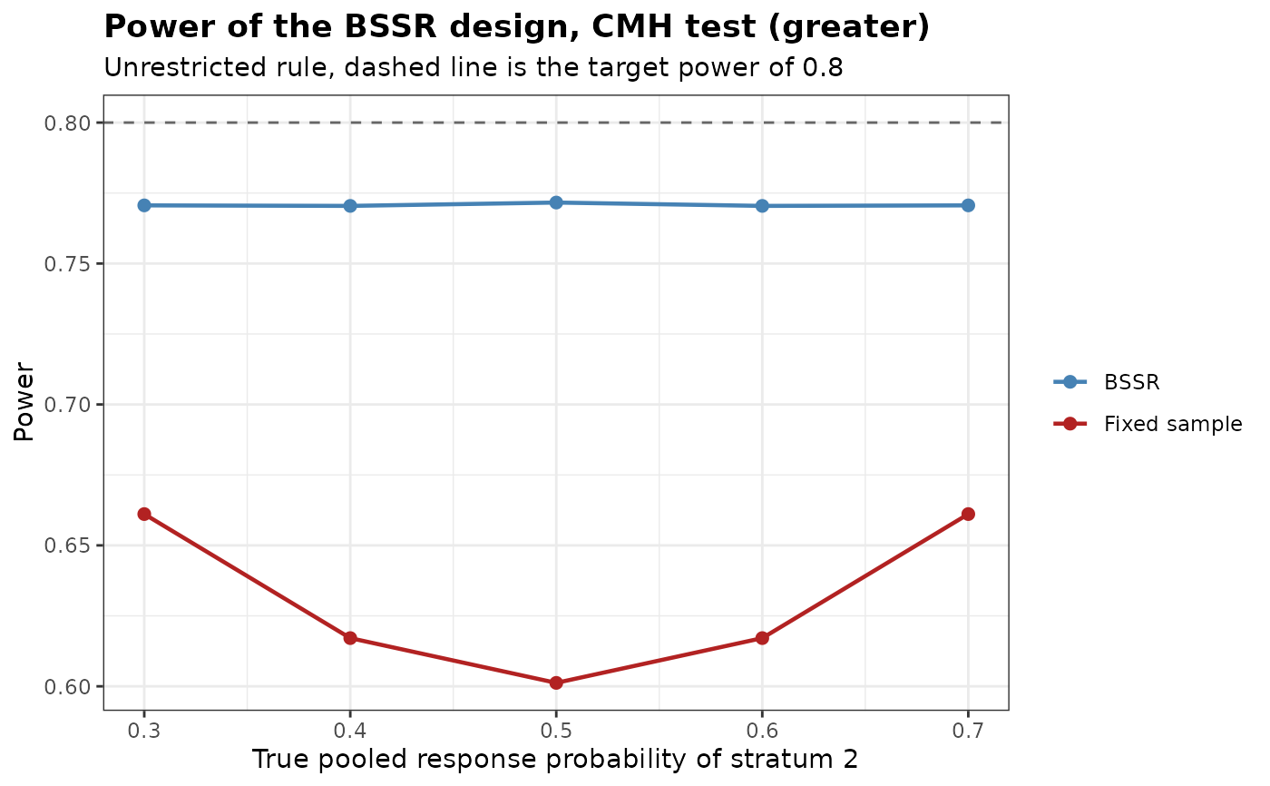
Plot the Power of a Stratified BSSR Design against the Fixed Design
Source:R/plot.bbssr_spowerbssr.R
plot.bbssr_spowerbssr.RdDraws the power of the design with blinded sample size re-estimation of
StratPowerBSSR and that of the fixed design against a chosen column of
the scenarios, as plot.bbssr_powerbssr does for two groups.
Usage
# S3 method for class 'bbssr_spowerbssr'
plot(x, x.by = NULL, xlab = NULL, ...)
Arguments
- x
An object of class
bbssr_spowerbssrreturned byStratPowerBSSR- x.by
Name of the numeric column of
xon the horizontal axis, or'scenario'for the rows ofpthat the scenarios come from. The default ofNULLtakes the first of the true pooled response probabilitiesp.S1, p.S2, ...that varies between the scenarios, or the scenario when none varies- xlab
Label of the horizontal axis.
NULLmakes it fromx.byand a singleNAdrops it- ...
Further arguments of
plot.bbssr_powerbssr:main,sub,ylab,ylim,ref.line,legend.title,legend.labels,show.points,coloursandbase_size
Details
The lines join the scenarios in the order of the horizontal axis, so the scenarios
should differ in a single probability, or x.by should name a column in which
they all differ; a warning is given when two scenarios share a value on the axis.
The Monte Carlo standard errors of a simulated or averaged power (three or more strata,
or a random allocation) are not drawn. With Delta.T = 0 in
StratPowerBSSR the curves are rejection probabilities under the null
hypothesis, and ref.line can be set to the level of significance.