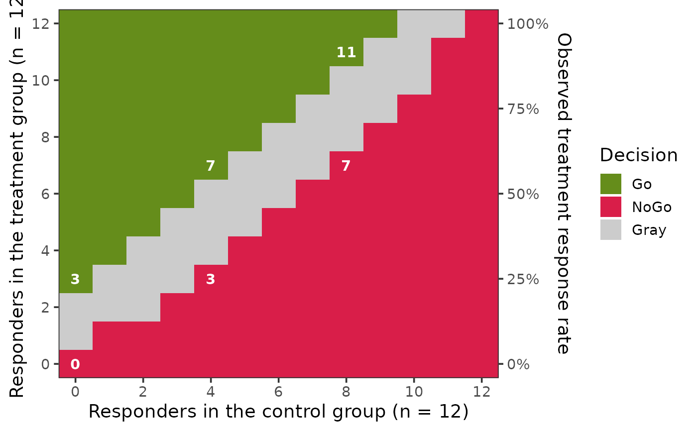
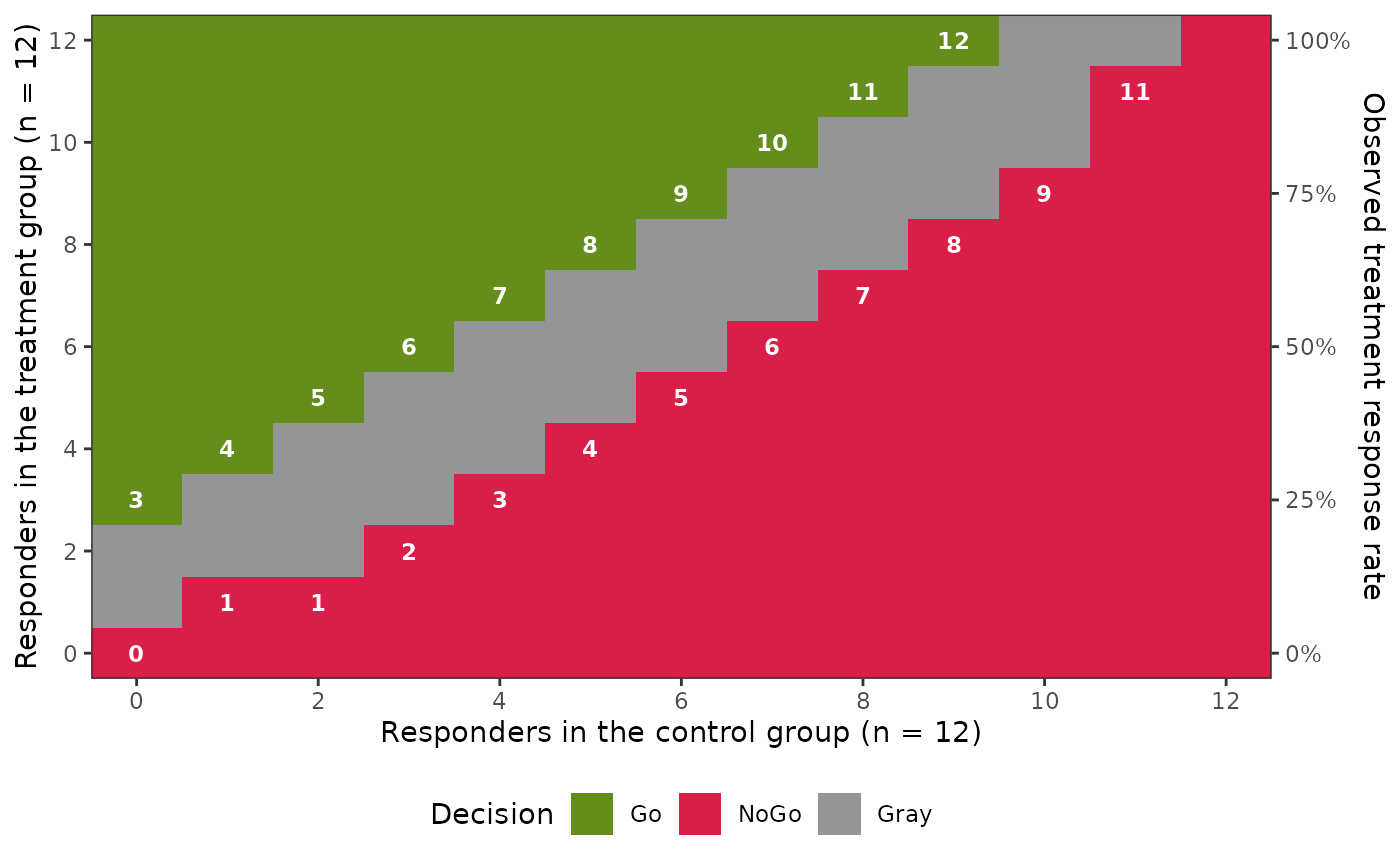
Plot a decision boundary — plot.qdm_boundary • BayesianQDM

Draws the decision intervals computed by qdm_boundary as regions filled by the decision (Go, NoGo, Gray, or Miss if it occurs): the horizontal axis is the condition (for example, the number of control responders or the treatment group size) and the vertical axis is the observed quantity (numbers of responders or events, or the observed treatment mean) or, for continuous endpoints with a concurrent control group, the observed difference in means. The boundary values are written on the Go and NoGo regions next to the boundaries, for example the smallest number of responders that leads to a Go decision. With a concurrent control group and a binary endpoint, the observed response rate of the treatment group is shown on a secondary axis.

Usage

# S3 method for class 'qdm_boundary'
plot(
  x,
  col_go = "#658D1B",
  col_nogo = "#D91E49",
  col_gray = "#939597",
  col_miss = "#E69F00",
  labels = TRUE,
  label_size = NULL,
  base_size = 11,
  legend_position = "bottom",
  ...
)

Arguments

x: An object of class "qdm_boundary".
col_go, col_nogo, col_gray, col_miss: Colors of the Go, NoGo, Gray and Miss decisions: color names or hexadecimal codes. The defaults are green, red, gray and orange. Transparency (an alpha value in the code) is not used in the heat maps.
labels: TRUE (the default) to write the boundary values for every value of the horizontal axis (or, with more than 16 values, for about six of them, leaving out the first and the last), FALSE for none, or a numeric vector of the values of the horizontal axis at which they are written.
label_size: Size of the boundary values, in millimeters, or NULL for the size of the axis tick labels, 0.8 * base_size / .pt.
base_size: Base font size of ggplot2::theme_bw(), in points, which sets the size of the axis labels, tick labels, legend and caption.
legend_position: Position of the legend: "bottom" (the default), "top", "left", "right" or "none". To place the legend inside the plot, add ggplot2::theme().
...: Not used; arguments given here are ignored with a warning.

Value

A ggplot object.

Details

The plot is a ggplot object, so it can be changed further by adding ggplot2 functions, for example ggplot2::labs(), ggplot2::theme() and ggplot2::scale_fill_manual().

Examples

des <- design_binary(
  n_t = 12, n_c = 12,
  prior_t = prior_beta(0.5, 0.5), prior_c = prior_beta(0.5, 0.5),
  criterion = criterion_posterior(theta_tv = 0.2, theta_mav = 0.1,
                                  gamma_go = 0.5, gamma_nogo = 0.8)
)
b <- qdm_boundary(des)
plot(b)

plot(b, labels = c(0, 4, 8), col_gray = "gray80", base_size = 14,
     legend_position = "right")