Decision boundary of a design

Finds the observed data that lead to each decision (Go, NoGo, Gray, or Miss) of a design: for example, how many responders out of \(n\) are needed for a Go decision, or how large the observed difference in means must be. Unlike the operating characteristics, the result does not depend on the true parameters. It is a table of decision intervals of an observed quantity (the numbers of responders or events, or an observed mean), one set of intervals for each value of a second quantity (the condition), together with the corresponding observed response rates, milestone survival probabilities and treatment effects. The intervals are printed as tables (print.qdm_boundary) and drawn as the regions of the decisions with the boundary values written on them (plot.qdm_boundary).

Usage

qdm_boundary(
  design,
  n_t = NULL,
  mean_t = NULL,
  sd_t = NULL,
  cov_t = NULL,
  events_t = NULL,
  exposure_t = NULL,
  data_c = NULL,
  seed = NULL
)

Arguments

design: A design created by design_binary, design_continuous, design_continuous2 or design_tte.
n_t: Numbers of subjects in the treatment group (whole numbers); by default that of the design. Several values are allowed for one binary endpoint without a concurrent control group and for one continuous endpoint. For a time-to-event endpoint, n_t only sets the default numbers of events.
mean_t: For one continuous endpoint, an optional numeric vector: the grid of observed treatment means on which the boundary values are searched. For two continuous endpoints, a list of two numeric vectors: the observed treatment means of endpoint 1 (the conditions) and the grid of observed treatment means of endpoint 2.
sd_t: Observed treatment standard deviations (one continuous endpoint; positive).
cov_t: Observed treatment covariance matrix (two continuous endpoints; a 2 x 2 positive definite matrix).
events_t: Numbers of events of the treatment group (time-to-event endpoint; whole numbers); by default 0:n_t.
exposure_t: Total observed times of the treatment group (time-to-event endpoint; positive).
data_c: Observed data of the concurrent control group, created by data_continuous, data_continuous2 or data_tte; required for those endpoints with a concurrent control group and NULL otherwise.
seed: Random seed for probabilities computed by Monte Carlo simulation, or NULL to use the current random number stream. If given, the previous state of the random number generator is restored on exit.

Value

An object of class c("qdm_boundary", "data.frame") with one row per decision interval and the columns

Conditions: n_t, n_c and y_c (binary; only n_t without a concurrent control group), n_t and sd_t (continuous), n_t, mean_t1 and effect1 (two continuous endpoints; the observed treatment mean of endpoint 1 and its difference from the control) or exposure_t (time-to-event).
decision: The decision (a factor with levels "Go", "NoGo", "Gray" and "Miss").
from, to: The ends of the interval of the observed quantity: the number of treatment responders or events (both ends included), or the observed treatment mean (of endpoint 2).
rate_from, rate_to: Binary endpoint: the observed response rates \(y_t / n_t\) at the ends.
surv_from, surv_to: Time-to-event endpoint evaluated by the milestone survival: the observed milestone survival probabilities \(\exp(-t_0 d_t / E_t)\) at the ends.
effect_from, effect_to: The observed treatment effect at the ends: the observed rate, mean or milestone survival minus that of the concurrent control group, or minus the fixed control value or the mean (location) of the distribution of the control group; for the hazard ratio, the observed hazard \(d_t / E_t\) divided by the observed control hazard (NA if the control group has no events), the fixed control hazard or the mean of the distribution of the control hazard. The values correspond to from and to, so effect_from is larger than effect_to when larger values of the observed quantity give smaller effects (for example, more events and the milestone survival).

The attributes design, axes, titles, increasing, discrete and range record the design and the information used by the print and plot methods.

Details

The observed quantity and the conditions depend on the endpoint:

One binary endpoint: The number of responders of the treatment group \(y_t = 0, \ldots, n_t\). With a concurrent control group, one set of intervals for each number of control responders \(y_c = 0, \ldots, n_c\) (n_t must be a single number; \(n_c\) is that of the design). Without one, one set for each sample size in n_t, which shows how the boundary changes with the sample size.
One continuous endpoint: The observed treatment mean, for each combination of sd_t and n_t (at most one of them may have more than one value). With a concurrent control group, data_c gives the observed control data. The boundary values are located by bisection between the values of a grid, mean_t or by default a grid of 201 values that covers the thresholds of the criterion.
Two continuous endpoints: The observed treatment mean of endpoint 2, located by bisection on the grid mean_t[[2]], for each observed treatment mean of endpoint 1 in mean_t[[1]], with the sample covariance matrix cov_t and n_t subjects (a single number). With a concurrent control group, data_c gives the observed control data.
One time-to-event endpoint: The number of events of the treatment group (events_t), for each total observed time in exposure_t. With a concurrent control group, data_c gives the observed control data.

Two binary endpoints are not supported, because their decision depends on the four cell counts and cannot be summarized by one observed quantity.

The decision for each value is made as in qdm_decide. For an observed mean, the first and last intervals extend to minus and plus infinity; changes of the decision beyond the grid (whose ends are extended by two values far beyond them) or two changes of the same criterion between two neighboring grid values are not detected. With a conjugate (Normal-Inverse-chi-squared) prior, the posterior scale increases with the distance between the observed mean and the prior mean, so the probability of the Go region need not increase with the observed mean; the intervals then show where it decreases again. Probabilities computed by Monte Carlo simulation (method = "MC", or posterior predictive probabilities of a time-to-event endpoint) make the boundary values approximate.

Examples

# Single-arm study with a fixed control response rate of 0.2: responders
# needed out of 10 to 30 subjects
des <- design_binary(
  n_t = 20, n_c = 0, prior_t = prior_beta(1, 1),
  criterion = criterion_posterior(theta_tv = 0.2, theta_mav = 0.05,
                                  gamma_go = 0.8, gamma_nogo = 0.8),
  fixed_c = 0.2
)
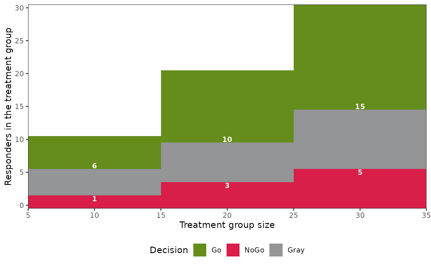
b <- qdm_boundary(des, n_t = c(10, 20, 30))
b
#> Decision boundary of a design with one binary endpoint
#> 
#> Responders in the treatment group (y_t)
#>   n_t   NoGo   Gray   Go
#>   10    0-1    2-5    6-10
#>   20    0-3    4-9    10-20
#>   30    0-5    6-14   15-30
#> 
#> Observed response rate (y_t / n_t)
#>   n_t   NoGo            Gray             Go
#>   10    0.0% to 10.0%   20.0% to 50.0%   60.0% to 100.0%
#>   20    0.0% to 15.0%   20.0% to 45.0%   50.0% to 100.0%
#>   30    0.0% to 16.7%   20.0% to 46.7%   50.0% to 100.0%
#> 
#> Observed difference from the fixed control rate (y_t / n_t - 0.2)
#>   n_t   NoGo               Gray          Go
#>   10    -0.2 to -0.1       0 to 0.3      0.4 to 0.8
#>   20    -0.2 to -0.05      0 to 0.25     0.3 to 0.8
#>   30    -0.2 to -0.03333   0 to 0.2667   0.3 to 0.8
plot(b)


# Continuous endpoint with a concurrent control group: observed
# differences in means needed for each observed standard deviation
des2 <- design_continuous(
  n_t = 12, n_c = 12,
  prior_t = prior_vague(), prior_c = prior_vague(),
  criterion = criterion_posterior(theta_tv = 30, theta_mav = 15,
                                  gamma_go = 0.6, gamma_nogo = 0.7),
  method = "MM"
)
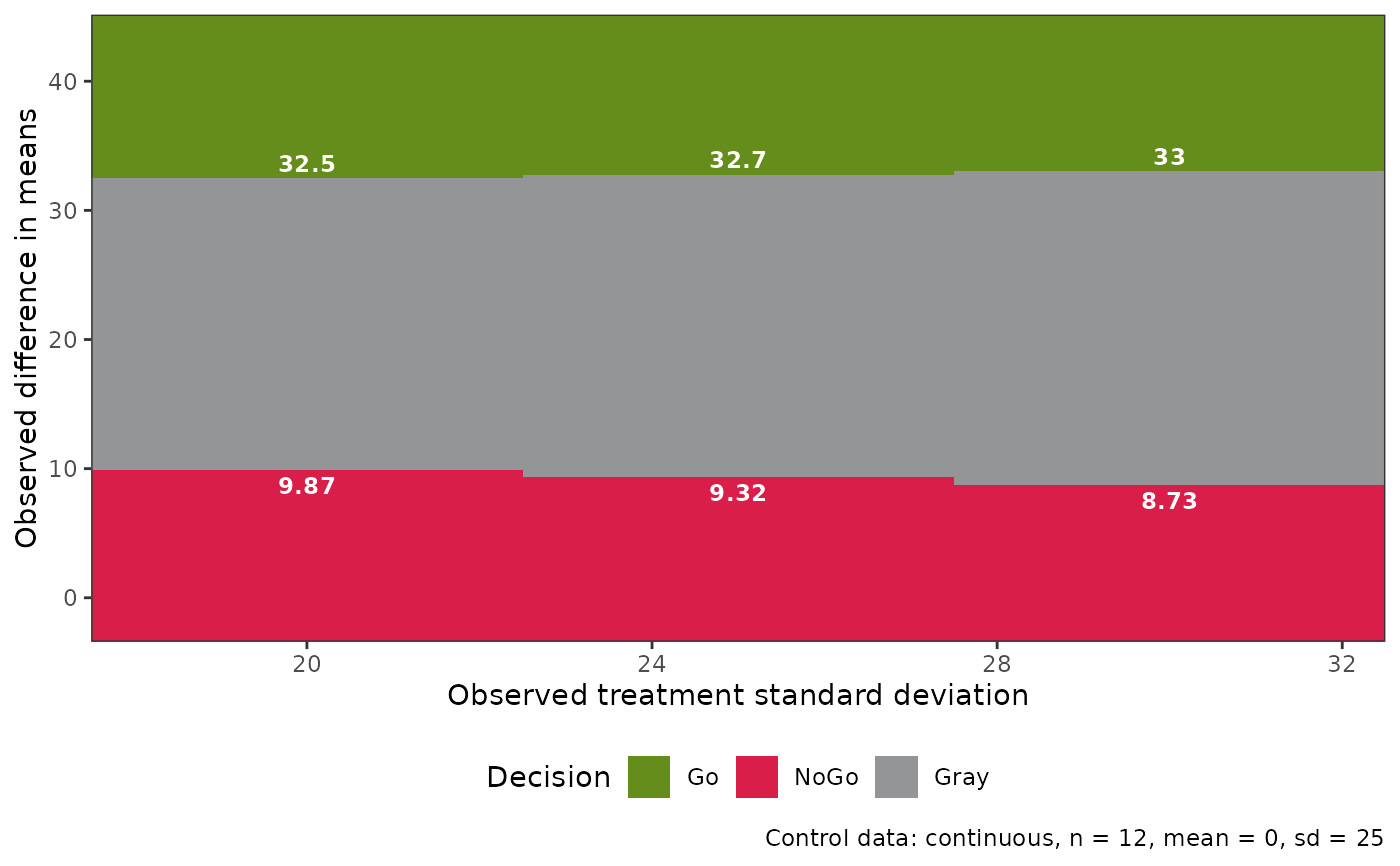
b2 <- qdm_boundary(des2, sd_t = c(20, 25, 30),
                   data_c = data_continuous(12, 0, 25))
b2
#> Decision boundary of a design with one continuous endpoint
#>   n_t = 12
#>   Control data: continuous, n = 12, mean = 0, sd = 25
#> 
#> Observed treatment mean
#>   sd_t   NoGo       Gray             Go
#>   20     <= 9.866   9.866 to 32.47   >= 32.47
#>   25     <= 9.321   9.321 to 32.74   >= 32.74
#>   30     <= 8.735   8.735 to 33.02   >= 33.02
#> 
#> Observed difference in means (control mean 0)
#>   sd_t   NoGo       Gray             Go
#>   20     <= 9.866   9.866 to 32.47   >= 32.47
#>   25     <= 9.321   9.321 to 32.74   >= 32.74
#>   30     <= 8.735   8.735 to 33.02   >= 33.02
plot(b2)

Usage

Arguments

Value

Details

See also

Examples