Time-to-event endpoint • BayesianQDM

This vignette describes the analysis of a proof-of-concept (PoC) study with one time-to-event endpoint, such as progression-free survival, evaluated by the survival probability at a milestone time or by the hazard ratio. vignette("overview") introduces the decision criteria.

Model

In group $k$ ( $k = t, c$ ), the event times are exponential with hazard $\lambda_k$ , and the data are summarized by the number of events $d_k$ and the total observed time $E_k$ , the sum of the follow-up times of all subjects until their event or censoring (data_tte()). With the Gamma prior $\lambda_k \sim \textrm{Gamma}(a_k, b_k)$ (shape $a_k$ and rate $b_k$ ; prior_gamma()), the posterior distribution is $\lambda_k \mid D \sim \textrm{Gamma}(a_k + d_k, \; b_k + E_k).$ The prior acts as $a_k$ events in a total observed time of $b_k$ , so a prior with a small shape and rate, such as prior_gamma(0.1, 1) with time in months, has little influence.

The effect is the difference of the survival probabilities at the milestone time $t_0$ , $\theta = S_t(t_0) - S_c(t_0), \qquad S_k(t_0) = \exp(-\lambda_k t_0).$ The posterior probability $\Pr(\theta > q \mid D)$ is computed by numerical integration over the control hazard (psurvdiff()).

Alternatively, the effect is the hazard ratio $\theta = \lambda_t / \lambda_c$ (effect = "hazard_ratio"; Huang et al., 2019). With the posterior shapes $a_k^* = a_k + d_k$ and rates $b_k^* = b_k + E_k$ , its posterior distribution is a scaled F distribution, $\frac{a_c^* b_t^*}{a_t^* b_c^*} \, \theta \mid D \sim F(2 a_t^*, 2 a_c^*),$ so its posterior probabilities are computed exactly (phazardratio()).

External data with $d_e$ events and total observed time $E_e$ enter through a power prior with weight $a_0$ , which adds $a_0 d_e$ to the shape and $a_0 E_e$ to the rate. A hypothetical control adds its events and total observed time to the prior of the control group.

Decision for observed data

A single-arm study is often compared with a known benchmark. With fixed_c, the control survival probability at the milestone is a known value $S_{c0}$ , and the probabilities of the Go and NoGo regions are Gamma probabilities of the treatment hazard. Consider 30 subjects, a milestone of 3 months, a benchmark of 0.72, $\theta_{TV} = 0.15$ and $\theta_{MAV} = 0$ :

crit <- criterion_posterior(theta_tv = 0.15, theta_mav = 0,
                            gamma_go = 0.6, gamma_nogo = 0.8)
des <- design_tte(n_t = 30, n_c = 0, prior_t = prior_gamma(0.1, 1),
                  criterion = crit, milestone = 3, fixed_c = 0.72)
dec <- qdm_decide(des, data_t = data_tte(events = 6, exposure = 150))
dec
#> Decision: Go
#>   Go:   P(theta > 0.15 | data) = 0.6863 (threshold 0.6, met)
#>   NoGo: P(theta <= 0 | data) = 0.001061 (threshold 0.8, not met)
#> Posterior distributions
#>   Treatment: hazard ~ Gamma(shape = 6.1, rate = 151)
#>   Control:   fixed value 0.72

The Go region is $S_t(3) > 0.72 + 0.15$ , that is $\lambda_t < -\log(0.87) / 3$ , whose posterior probability is

pgamma(-log(0.87) / 3, shape = 0.1 + 6, rate = 1 + 150)
#> [1] 0.6862592

With fixed_c = 0, the effect is the milestone survival probability itself, and the thresholds are survival probabilities.

With a concurrent control group of 30 subjects:

des_c <- design_tte(n_t = 30, n_c = 30, prior_t = prior_gamma(0.1, 1),
                    prior_c = prior_gamma(0.1, 1), criterion = crit,
                    milestone = 3)
dec_c <- qdm_decide(des_c, data_t = data_tte(6, 150),
                    data_c = data_tte(12, 140))
dec_c
#> Decision: Gray
#>   Go:   P(theta > 0.15 | data) = 0.2906 (threshold 0.6, not met)
#>   NoGo: P(theta <= 0 | data) = 0.05513 (threshold 0.8, not met)
#> Posterior distributions
#>   Treatment: hazard ~ Gamma(shape = 6.1, rate = 151)
#>   Control:   hazard ~ Gamma(shape = 12.1, rate = 141)
post_t <- dec_c$posterior_t
post_c <- dec_c$posterior_c
psurvdiff(0.15, milestone = 3, shape_t = post_t[["shape"]],
          rate_t = post_t[["rate"]], shape_c = post_c[["shape"]],
          rate_c = post_c[["rate"]], lower.tail = FALSE)
#> [1] 0.2905515

External control data and hypothetical controls are given as in the other vignettes, with borrow(data_tte(...), a0) and hypothetical(data_tte(...)).

Conduct of the study

The operating characteristics and the predictive criterion need the timing of the study, which conduct_tte() specifies: the enrollment (piecewise uniform over the intervals of accrual_time with relative rates accrual_rate), the dropout (piecewise exponential hazards) and the time of the analysis, either at a calendar time (cut_time) or at the time of a given number of events among all subjects of the study (cut_events). For example, enrollment over 15 months with increasing rates, a small dropout hazard and an analysis 15.44 months after the start of enrollment:

cond <- conduct_tte(accrual_time = c(0, 5, 10, 15),
                    accrual_rate = c(0.4, 2, 4.5),
                    dropout_hazard = 0.00226, cut_time = 15.44)
cond
#> Enrollment: piecewise uniform on (0, 5, 10, 15) with rates (0.4, 2.0, 4.5)
#> Dropout: hazard 0.00226
#> Analysis: at time 15.44
des <- design_tte(n_t = 30, n_c = 0, prior_t = prior_gamma(0.1, 1),
                  criterion = crit, milestone = 3, conduct = cond,
                  fixed_c = 0.72)

Predictive criterion

For the predictive criterion, a future study with $m_t$ and $m_c$ subjects is conducted as specified by conduct_future (by default conduct). The survival probability of each group in the future study is estimated by $\exp\{-t_0 (a + \tilde d) / (b + \tilde E)\}$ , from its number of events $\tilde d$ and total observed time $\tilde E$ , and the future effect is the difference of the two estimates (or the treatment estimate minus the fixed value). The predictive probabilities are estimated by simulating nMC future studies, each with hazards drawn from the posterior distributions, so they are Monte Carlo estimates and depend on the seed:

des_pred <- design_tte(
  n_t = 30, n_c = 0, prior_t = prior_gamma(0.1, 1),
  criterion = criterion_predictive(theta_null = 0.05, m_t = 60,
                                   gamma_go = 0.8, gamma_nogo = 0.3),
  milestone = 3, conduct = cond, fixed_c = 0.72, nMC = 5000
)
qdm_decide(des_pred, data_t = data_tte(6, 150), seed = 1)
#> Decision: Go
#>   Go:   P(future theta > 0.05 | data) = 0.9682 (threshold 0.8, met)
#>   NoGo: P(future theta <= 0.05 | data) = 0.0318 (threshold 0.3, not met)
#> Posterior distributions
#>   Treatment: hazard ~ Gamma(shape = 6.1, rate = 151)
#>   Control:   fixed value 0.72

Operating characteristics

A scenario gives the median survival time of each group (median_t and, with a concurrent control group, median_c), and the hazard is $\log 2$ divided by the median. qdm_oc() simulates nsim studies conducted as specified by conduct, with the same random numbers for all scenarios. The median for which the milestone survival equals the benchmark is med0 below, and the median for which it equals the benchmark plus $\theta_{TV}$ is med1:

med0 <- 3 * log(2) / -log(0.72)
med1 <- 3 * log(2) / -log(0.72 + 0.15)
c(med0, med1)
#> [1]  6.330033 14.931859
scen <- data.frame(median_t = c(6, 8, 10, 12, 15, 20))
oc <- qdm_oc(des, scen, seed = 1)
oc
#> Operating characteristics (simulation of 10000 studies; probabilities by exact computation (fixed control))
#>  median_t     Go   NoGo   Gray Miss
#>         6 0.0035 0.2252 0.7713    0
#>         8 0.0384 0.0435 0.9181    0
#>        10 0.1284 0.0083 0.8633    0
#>        12 0.2671 0.0018 0.7311    0
#>        15 0.4681 0.0002 0.5317    0
#>        20 0.7152 0.0000 0.2848    0
plot(oc)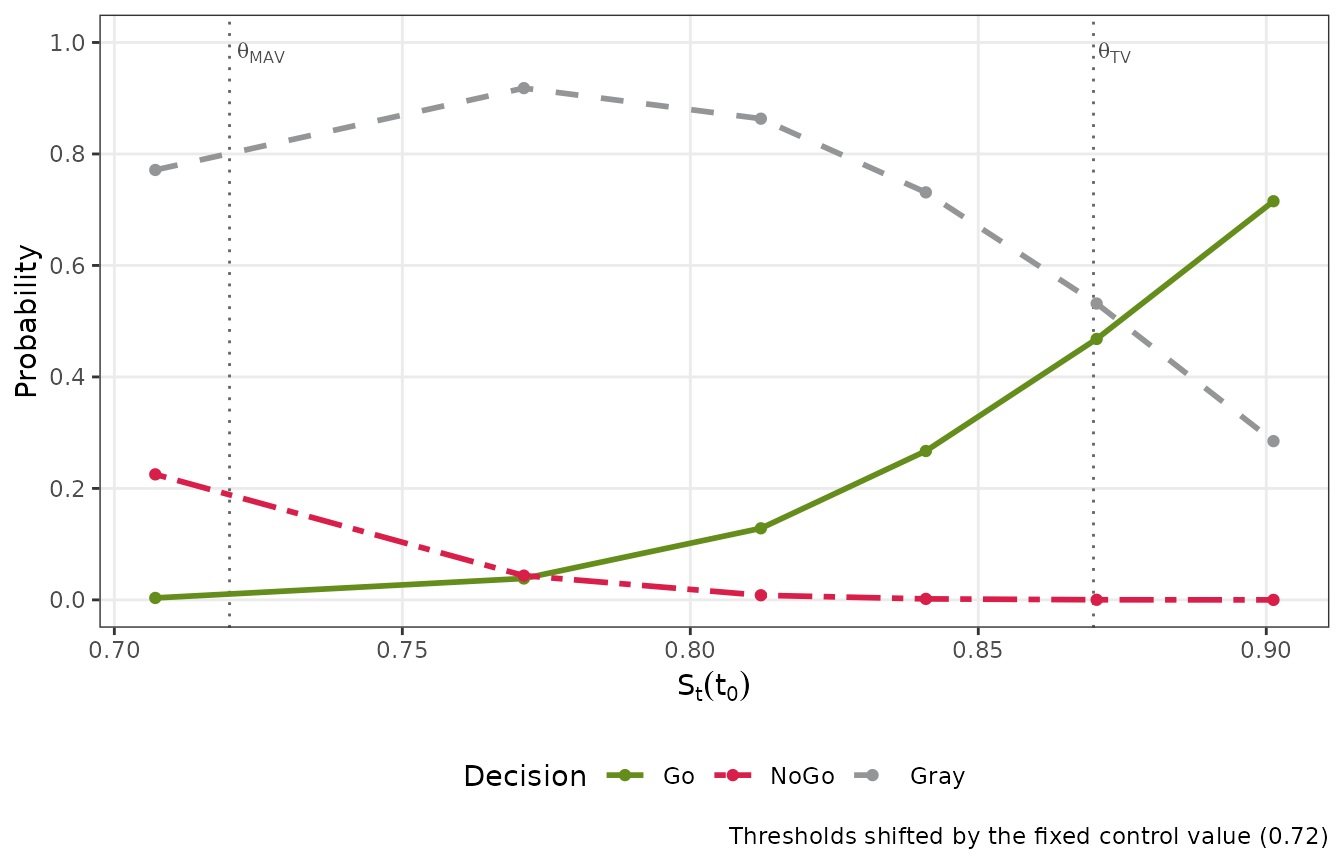

The horizontal axis is the survival probability of the treatment group at the milestone, and the vertical lines are shifted by the fixed control value. For a design with a concurrent control group, the probabilities of each simulated study are computed by numerical integration, which takes longer; here 1000 studies are simulated per scenario:

des_c <- design_tte(n_t = 30, n_c = 30, prior_t = prior_gamma(0.1, 1),
                    prior_c = prior_gamma(0.1, 1), criterion = crit,
                    milestone = 3, conduct = cond)
oc_c <- qdm_oc(des_c, data.frame(median_t = c(med0, 10, 15, 20),
                                 median_c = med0), nsim = 1000, seed = 1)
oc_c
#> Operating characteristics (simulation of 1000 studies; probabilities by numerical integration)
#>  median_t median_c    Go  NoGo  Gray Miss
#>      6.33     6.33 0.033 0.193 0.774    0
#>     10.00     6.33 0.183 0.033 0.784    0
#>     15.00     6.33 0.389 0.002 0.609    0
#>     20.00     6.33 0.530 0.002 0.468    0

With a predictive criterion, every simulated study requires nMC simulated future studies, so small values of nsim and nMC are advisable for exploration.

Calibration of the thresholds

The thresholds of the single-arm design are calibrated so that the Go criterion is met with probability at most 0.05 when the milestone survival equals the benchmark (median med0), and the NoGo criterion with probability at most 0.1 when it equals the benchmark plus 0.15 (median med1):

cal <- qdm_calibrate(des, scenario_go = data.frame(median_t = med0),
                     scenario_nogo = data.frame(median_t = med1),
                     target_go = 0.05, target_nogo = 0.1, seed = 1)
cal
#> Calibration of the decision thresholds (simulation of 10000 studies; probabilities by exact computation (fixed control))
#>   gamma_go   = 0.24: P(Go criterion met | scenario_go) = 0.0489 (target 0.05)
#>   gamma_nogo = 0.1: P(NoGo criterion met | scenario_nogo) = 0.0928 (target 0.1)
#> Decision probabilities with the chosen thresholds
#>       scenario median_t     Go   NoGo   Gray Miss
#>    scenario_go     6.33 0.0489 0.8815 0.0696    0
#>  scenario_nogo    14.93 0.7995 0.0928 0.1077    0
plot(cal)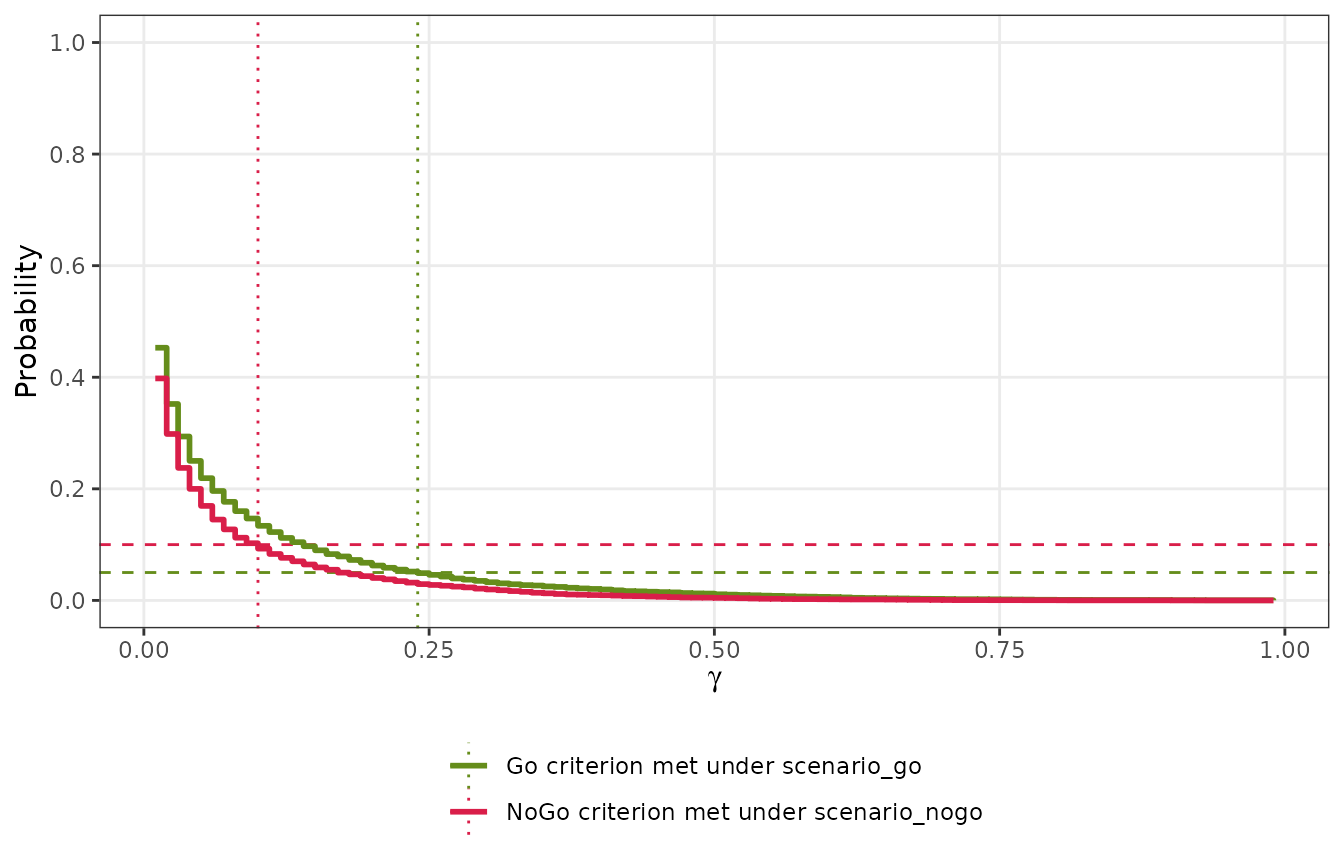

The chosen thresholds are $\gamma_{go} =$ 0.24 and $\gamma_{nogo} =$ 0.1.

Decision boundary

qdm_boundary() gives, for each total observed time of the treatment group, the numbers of events that lead to Go, NoGo and Gray decisions, with the corresponding observed milestone survival probabilities $\exp(-t_0 d_t / E_t)$ and observed effects. With a posterior criterion, it does not depend on the conduct of the study:

b <- qdm_boundary(des, exposure_t = seq(100, 300, by = 50))
b
#> Decision boundary of a design with one time-to-event endpoint (milestone survival)
#> 
#> Events in the treatment group (d_t)
#>   exposure_t   Go     Gray    NoGo
#>   100          0-4    5-14    15-30
#>   150          0-6    7-20    21-30
#>   200          0-8    9-26    27-30
#>   250          0-11   12-30   -
#>   300          0-13   14-30   -
#> 
#> Observed milestone survival exp(-3 d_t / E_t)
#>   exposure_t   Go            Gray               NoGo
#>   100          0.8869 to 1   0.657 to 0.8607    0.4066 to 0.6376
#>   150          0.8869 to 1   0.6703 to 0.8694   0.5488 to 0.657
#>   200          0.8869 to 1   0.6771 to 0.8737   0.6376 to 0.667
#>   250          0.8763 to 1   0.6977 to 0.8659   -
#>   300          0.8781 to 1   0.7408 to 0.8694   -
#> 
#> Observed difference in milestone survival (control 0.72, fixed control value)
#>   exposure_t   Go               Gray                 NoGo
#>   100          0.1669 to 0.28   -0.06295 to 0.1407   -0.3134 to -0.08237
#>   150          0.1669 to 0.28   -0.04968 to 0.1494   -0.1712 to -0.06295
#>   200          0.1669 to 0.28   -0.04294 to 0.1537   -0.08237 to -0.05302
#>   250          0.1563 to 0.28   -0.02232 to 0.1459   -
#>   300          0.1581 to 0.28   0.02082 to 0.1494    -

With a total observed time of 150 months, a Go decision needs at most 6 events. The plot shows the regions of the decisions over many values of the total observed time:

plot(qdm_boundary(des, exposure_t = seq(20, 400, by = 5)))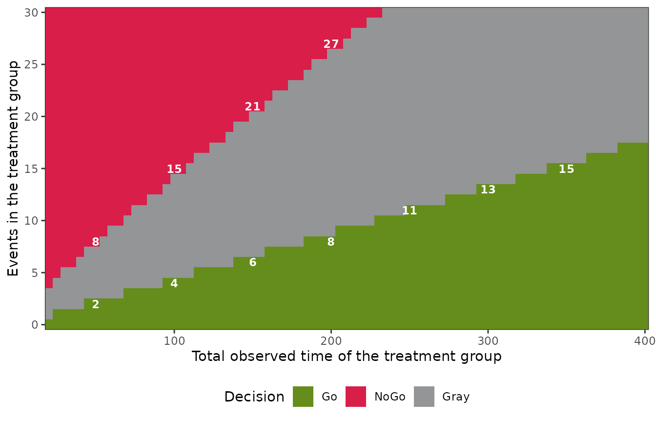

For a design with a concurrent control group, the observed control data are given by data_c.

Hazard ratio

With effect = "hazard_ratio", smaller effects are favorable, so the criterion is specified with direction = "less": the Go region is $\theta < \theta_{TV}$ and the NoGo region is $\theta \ge \theta_{MAV}$ , with $\theta_{TV} < \theta_{MAV}$ . The example of Huang et al. (2019) is a randomized study with 112 subjects in the treatment group and 56 in the control group, uniform enrollment over 13 months, a control median survival time of 8.5 months, a loss-to-follow-up hazard of 0.003 per month, a target value of 0.67 and a minimum acceptable value of 0.8 for the hazard ratio, and an analysis at 127 events. Huang et al. (2019) use the minimum acceptable value in their Go rule, as a bound for the upper confidence limit of the hazard ratio. Here the decision is Go if the hazard ratio is below 0.67 with probability at least 0.5, and NoGo if it is at least 0.8 with probability at least 0.6:

crit_hr <- criterion_posterior(theta_tv = 0.67, theta_mav = 0.8,
                               gamma_go = 0.5, gamma_nogo = 0.6,
                               direction = "less")
des_hr <- design_tte(
  n_t = 112, n_c = 56, prior_t = prior_gamma(0.01, 0.01),
  prior_c = prior_gamma(0.01, 0.01), criterion = crit_hr,
  effect = "hazard_ratio",
  conduct = conduct_tte(accrual_time = c(0, 13), dropout_hazard = 0.003,
                        cut_events = 127)
)
dec_hr <- qdm_decide(des_hr, data_t = data_tte(75, 1100),
                     data_c = data_tte(52, 420))
dec_hr
#> Decision: Go
#>   Go:   P(theta < 0.67 | data) = 0.8569 (threshold 0.5, met)
#>   NoGo: P(theta >= 0.8 | data) = 0.02137 (threshold 0.6, not met)
#> Posterior distributions
#>   Treatment: hazard ~ Gamma(shape = 75.01, rate = 1100)
#>   Control:   hazard ~ Gamma(shape = 52.01, rate = 420)
post_t <- dec_hr$posterior_t
post_c <- dec_hr$posterior_c
phazardratio(0.67, shape_t = post_t[["shape"]], rate_t = post_t[["rate"]],
             shape_c = post_c[["shape"]], rate_c = post_c[["rate"]])
#> [1] 0.8569464

The argument milestone is not used and must not be given. Under the exponential model, the hazard ratio is the ratio of the median survival times of the control and treatment groups, which is the horizontal axis of the plot of operating characteristics:

oc_hr <- qdm_oc(des_hr, data.frame(median_t = 8.5 / c(0.5, 0.6, 0.7, 0.8, 1),
                                   median_c = 8.5), seed = 1)
oc_hr
#> Operating characteristics (simulation of 10000 studies; probabilities by exact computation (F distribution))
#>  median_t median_c     Go   NoGo   Gray Miss
#>     17.00      8.5 0.9433 0.0017 0.0550    0
#>     14.17      8.5 0.7204 0.0358 0.2438    0
#>     12.14      8.5 0.4108 0.1685 0.4207    0
#>     10.62      8.5 0.1702 0.3985 0.4313    0
#>      8.50      8.5 0.0176 0.8258 0.1566    0
plot(oc_hr)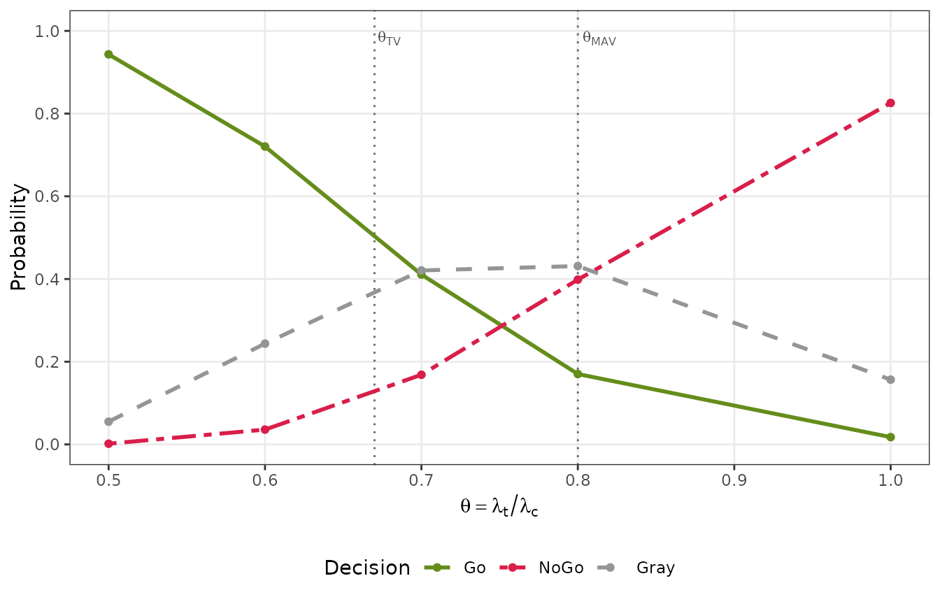

The probabilities of a Go decision are close to those of Table 1 of Huang et al. (2019), which are based on the normal approximation of the estimated log hazard ratio (0.946, 0.727, 0.406 and 0.170 for hazard ratios of 0.5, 0.6, 0.7 and 0.8). The decision boundary gives the numbers of treatment events that lead to each decision for given total observed times of the treatment group and given control data (data_c), with the observed hazard ratios $(d_t / E_t) / (d_c / E_c)$ :

qdm_boundary(des_hr, exposure_t = seq(800, 1400, by = 200),
             data_c = data_tte(52, 420))
#> Decision boundary of a design with one time-to-event endpoint (hazard ratio)
#>   Control data: time-to-event, events = 52, exposure = 420
#> 
#> Events in the treatment group (d_t)
#>   exposure_t   Go      Gray      NoGo
#>   800          0-66    67-82     83-112
#>   1000         0-82    83-103    104-112
#>   1200         0-99    100-112   -
#>   1400         0-112   -         -
#> 
#> Observed hazard ratio: d_t / E_t divided by the control hazard 0.1238 (observed in the control group)
#>   exposure_t   Go            Gray               NoGo
#>   800          0 to 0.6663   0.6764 to 0.8279   0.838 to 1.131
#>   1000         0 to 0.6623   0.6704 to 0.8319   0.84 to 0.9046
#>   1200         0 to 0.6663   0.6731 to 0.7538   -
#>   1400         0 to 0.6462   -                  -

For a single-arm study, fixed_c is the median survival time of the control, whose hazard is $\log 2$ divided by it. For the predictive criterion, the hazard of each group in the future study is estimated by $(a + \tilde d) / (b + \tilde E)$ , the future effect is the ratio of the two estimates, and with direction = "less" the Go region is that it is below $\theta_{NULL}$ .

Reference

Huang, B., Talukder, E., Han, L. and Kuan, P.-F. (2019). Quantitative decision-making in randomized Phase II studies with a time-to-event endpoint. Journal of Biopharmaceutical Statistics, 29(1), 189–202. https://doi.org/10.1080/10543406.2018.1489400