Operating characteristics of a design

Computes the probabilities of Go, NoGo, Gray and Miss decisions of a design under scenarios for the true parameters.

Usage

qdm_oc(design, scenarios, nsim = 10000L, seed = NULL)

Arguments

design: A design created by design_binary, design_continuous, design_binary2, design_continuous2 or design_tte.
scenarios: A data frame with one row per scenario. For a binary endpoint the columns pi_t and pi_c give the true response rates of the treatment and control groups. For a continuous endpoint the columns mu_t, sd_t, mu_c and sd_c give the true means and standard deviations. For two binary endpoints the columns pi_t1, pi_t2, rho_t, pi_c1, pi_c2 and rho_c give the true response rates of endpoints 1 and 2 (strictly between 0 and 1) and the correlation of the two endpoints in each group. For two continuous endpoints the columns mu_t1, mu_t2, sd_t1, sd_t2, rho_t, mu_c1, mu_c2, sd_c1, sd_c2 and rho_c give the true means, standard deviations and correlation of the two endpoints in each group (the correlation strictly between -1 and 1). For a time-to-event endpoint the columns median_t and median_c give the true median survival times (positive). The columns of the control group are not needed for a design without a concurrent control group. Other columns, such as labels, are kept in the result.
nsim: Number of simulated studies per scenario for designs whose operating characteristics are computed by simulation.
seed: Random seed for the simulation and for Monte Carlo estimates of probabilities, or NULL to use the current random number stream. If given, the previous state of the random number generator is restored on exit.

Value

An object of class c("qdm_oc", "data.frame"): the scenarios with the columns Go, NoGo, Gray and Miss added. The attributes design and method record the design and the method of computation.

Details

For a binary endpoint, all possible outcomes of the proof-of-concept study are enumerated and the probabilities are exact (Kang et al., 2026, Section 4.3); nsim and seed are not used.

For a continuous endpoint, nsim studies are simulated under each scenario. Only the sufficient statistics are simulated: the sample mean \(\bar y = \mu + \sigma Z / \sqrt{n}\) and the sample standard deviation \(s = \sigma \sqrt{X / (n - 1)}\), with \(Z \sim N(0, 1)\) and \(X \sim \chi^2_{n - 1}\). The same random numbers are used for all scenarios, so the results change smoothly across scenarios. The probabilities have a simulation standard error of at most \(0.5 / \sqrt{nsim}\) (0.005 for the default nsim). For each simulated study, the probabilities of the Go and NoGo regions are computed by the method of the design (see design_continuous), of which method = "MM" is the fastest. To explore many scenarios or designs, method = "MM" or a smaller nsim gives results quickly; the chosen design can then be checked with method = "NI" and the default nsim.

For two binary endpoints, all outcomes are enumerated (Yamaguchi et al., submitted, equation A.5) or nsim studies are simulated, as specified by enumerate in design_binary2. The response rates and correlation of each group are converted to cell probabilities by cellprob_binary2; a scenario whose correlation is outside the feasible range for its response rates is not evaluable, and its probabilities are NA (with a warning).

For two continuous endpoints, nsim studies are simulated under each scenario. Only the sufficient statistics are simulated: the sample means \(\bar y = \mu + L z / \sqrt{n}\) and the matrix of sums of squares and cross-products \(S = L A A^T L^T\), where \(L\) is the Cholesky factor of the covariance matrix of the scenario, \(z\) has two independent standard normal elements and \(A\) is the Bartlett factor of a Wishart distribution with \(n - 1\) degrees of freedom. The same random numbers are used for all scenarios.

For a time-to-event endpoint, nsim studies are simulated under each scenario as specified by the conduct of the design (enrollment, dropout and analysis time; see conduct_tte), with exponential event times whose hazard is \(\log(2) / M\) for the median survival time \(M\) of the scenario. The same random numbers are used for all scenarios. With a predictive criterion, every simulated study needs nMC simulated future studies (see design_tte), so the computing time grows with nsim times nMC.

The decision for each outcome is made as in qdm_decide. A warning is given when Miss decisions (both criteria met) have positive probability in some scenario.

References

Kang, R., Yamaguchi, Y. and Han, C. (2026). Bayesian quantitative decision-making framework in cell and gene therapy development for rare diseases. Journal of Biopharmaceutical Statistics. doi:10.1080/10543406.2026.2655410

Yamaguchi, Y., Hu, H., Huang, Y., Han, C., Homma, G. and Wang, A. (submitted). Bivariate Bayesian quantitative decision-making for two endpoints in rare disease drug development.

Examples

des <- design_binary(
  n_t = 12, n_c = 12,
  prior_t = prior_beta(0.5, 0.5), prior_c = prior_beta(0.5, 0.5),
  criterion = criterion_posterior(theta_tv = 0.2, theta_mav = 0.1,
                                  gamma_go = 0.5, gamma_nogo = 0.8)
)
oc <- qdm_oc(des, data.frame(pi_t = seq(0.2, 0.8, by = 0.1), pi_c = 0.4))
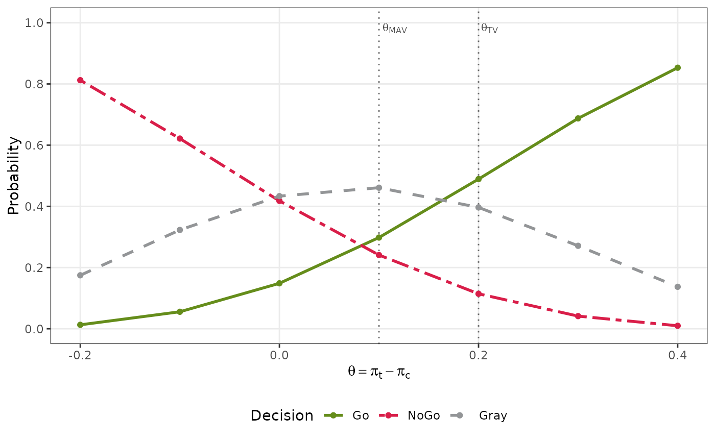
oc
#> Operating characteristics (exact enumeration of the outcomes)
#>  pi_t pi_c      Go     NoGo   Gray Miss
#>   0.2  0.4 0.01290 0.812335 0.1748    0
#>   0.3  0.4 0.05552 0.621598 0.3229    0
#>   0.4  0.4 0.14854 0.417981 0.4335    0
#>   0.5  0.4 0.29810 0.240949 0.4610    0
#>   0.6  0.4 0.48908 0.114276 0.3966    0
#>   0.7  0.4 0.68750 0.041368 0.2711    0
#>   0.8  0.4 0.85307 0.009801 0.1371    0
plot(oc)


# Continuous endpoint (moment-matching approximation for speed)
des2 <- design_continuous(
  n_t = 12, n_c = 12,
  prior_t = prior_vague(), prior_c = prior_vague(),
  criterion = criterion_posterior(theta_tv = 30, theta_mav = 15,
                                  gamma_go = 0.6, gamma_nogo = 0.7),
  method = "MM"
)
oc2 <- qdm_oc(des2, data.frame(mu_t = seq(0, 50, by = 10), sd_t = 25,
                               mu_c = 0, sd_c = 25),
              nsim = 2000, seed = 1)
oc2
#> Operating characteristics (simulation of 2000 studies; probabilities by moment-matching approximation)
#>  mu_t sd_t mu_c sd_c     Go   NoGo   Gray Miss
#>     0   25    0   25 0.0010 0.8205 0.1785    0
#>    10   25    0   25 0.0165 0.4800 0.5035    0
#>    20   25    0   25 0.1130 0.1640 0.7230    0
#>    30   25    0   25 0.3915 0.0275 0.5810    0
#>    40   25    0   25 0.7530 0.0010 0.2460    0
#>    50   25    0   25 0.9450 0.0005 0.0545    0

# Two binary endpoints (small nMC for speed)
des3 <- design_binary2(
  n_t = 6, n_c = 6,
  prior_t = prior_dirichlet(rep(0.25, 4)),
  prior_c = prior_dirichlet(rep(0.25, 4)),
  criterion = criterion_posterior(theta_tv = c(0.15, 0.15),
                                  theta_mav = c(0.10, 0.10),
                                  gamma_go = 0.3, gamma_nogo = 0.4),
  nMC = 2000
)
effects <- expand.grid(theta1 = c(0, 0.15, 0.3), theta2 = c(0, 0.15, 0.3))
oc3 <- qdm_oc(des3, data.frame(pi_t1 = 0.2 + effects$theta1,
                               pi_t2 = 0.2 + effects$theta2, rho_t = 0.3,
                               pi_c1 = 0.2, pi_c2 = 0.2, rho_c = 0.3),
              seed = 1)
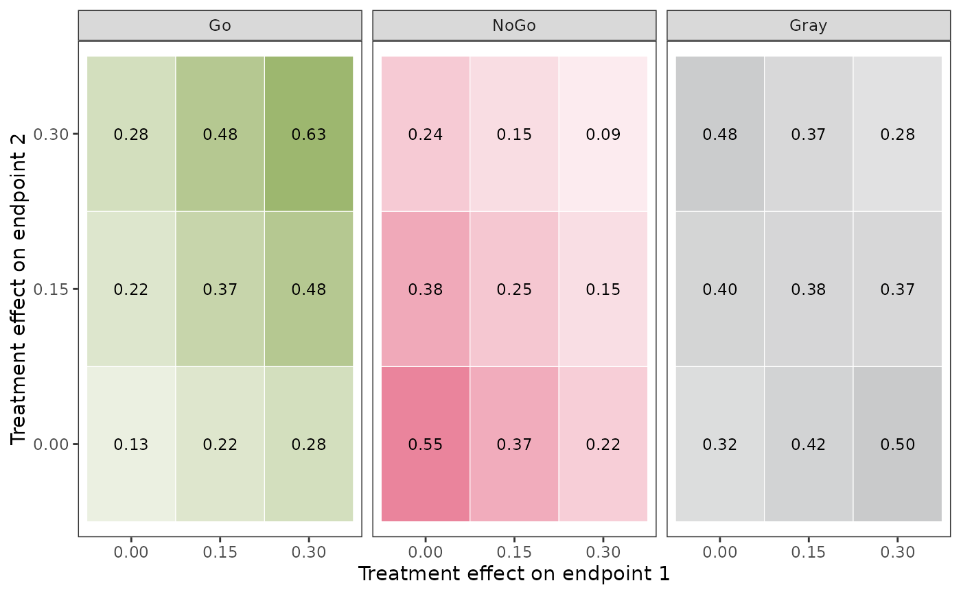
oc3
#> Operating characteristics (exact enumeration of the outcomes; posterior probabilities by Monte Carlo simulation (nMC = 2000))
#>  pi_t1 pi_t2 rho_t pi_c1 pi_c2 rho_c     Go    NoGo   Gray Miss
#>   0.20  0.20   0.3   0.2   0.2   0.3 0.1314 0.54527 0.3233    0
#>   0.35  0.20   0.3   0.2   0.2   0.3 0.2172 0.36700 0.4158    0
#>   0.50  0.20   0.3   0.2   0.2   0.3 0.2829 0.21711 0.5000    0
#>   0.20  0.35   0.3   0.2   0.2   0.3 0.2178 0.38223 0.4000    0
#>   0.35  0.35   0.3   0.2   0.2   0.3 0.3668 0.25104 0.3822    0
#>   0.50  0.35   0.3   0.2   0.2   0.3 0.4805 0.14661 0.3728    0
#>   0.20  0.50   0.3   0.2   0.2   0.3 0.2844 0.23534 0.4802    0
#>   0.35  0.50   0.3   0.2   0.2   0.3 0.4821 0.15235 0.3656    0
#>   0.50  0.50   0.3   0.2   0.2   0.3 0.6335 0.08806 0.2784    0
plot(oc3)